

1. Introduction
Steel pipe piles and related marine structures are exposed to chloride-rich water, oxygen, humidity, and temperature changes throughout their service life. The resulting corrosion reduces section thickness and, over time, may impair structural performance. Reliable estimates of corrosion development are therefore needed for corrosion allowance, inspection planning, maintenance, life-cycle costing, and service-life assessment (Melchers, 2003a, 2003b; Melchers & Jeffrey, 2008).
Marine corrosion does not progress at a constant rate. It is influenced by electrochemical reactions, oxygen and chloride transport, moisture, corrosion-product formation, localized attack, and environmental variability (Melchers, 2003a, 2003b; Melchers & Jeffrey, 2008). Bare steel may corrode rapidly at first. As corrosion products accumulate, they can restrict transport to the steel surface and slow the average rate, although cracking or spalling of the rust layer may later change that trend. A straight-line extrapolation is therefore unlikely to describe long-term behaviour adequately.
Long natural-exposure records are scarce because marine tests lasting several decades are costly and difficult to maintain (Andrade & Alonso, 1996; Wei et al., 2024). Accelerated testing provides observations within a practical laboratory period, but the resulting series are usually short, unevenly spaced, and uncertain, especially after conversion to equivalent exposure time. These features make long-range forecasting difficult.
Corrosion loss is often represented by power-law, exponential, or Weibull-type functions because these models are straightforward to calibrate and interpret (Le et al., 2026; Noor et al., 2007, 2013; Qin & Cui, 2003; Weibull, 1951). Their prescribed forms, however, may not reproduce changes in curvature and can become unreliable when extrapolated far beyond the calibration range.
Machine-learning and neural-network methods have been used to model corrosion rate, pitting, atmospheric exposure, and corrosion detection (Cavanaugh et al., 2010; Coelho et al., 2022; Dong et al., 2024; Hacıefendioğlu et al., 2025; Jung & Kim, 2025; Khadom et al., 2020; Narayana et al., 2025; Yang et al., 2024). These methods can capture complex nonlinear relationships when sufficiently large and representative datasets are available. The present corrosion series contains only a few time points and no broad set of explanatory variables; under such conditions, a flexible data-driven model may fit the observations but remain unreliable outside the calibration range.
Physics-informed learning can reduce this problem by enforcing mechanistic conditions during training. Even so, most such models still need more observations and input variables than are available in the present dataset, and their extrapolation may be hard to interpret. Grey models offer a simpler alternative for short, irregular time series because they use accumulated-sequence regularization and only a small number of parameters. This is not a general claim that grey models outperform machine learning; it reflects the constraints of the present dataset.
Grey System Theory was developed for systems with limited and incomplete information (Julong, 1989; Liu & Forrest, 2010). The Nonlinear Grey Bernoulli Model (NGBM) extends the basic grey formulation through a nonlinear exponent, allowing the fitted trajectory to adjust its curvature while retaining a compact parameter set.
Long-term NGBM extrapolation is not automatically stable. Near singular parameter regions, a solution that fits the calibration points can become negative, non-monotonic, complex, or excessively large outside that range. Physical constraints are therefore needed in addition to a conventional fitting criterion.
This study examines a constrained NGBM for forecasting cumulative corrosion mass loss in SKK490 steel coupons representing steel pipe material. Candidate solutions are screened for numerical stability and physical admissibility, and uncertainty is estimated with a parametric bootstrap.
Measurements corresponding to 4.5–30 years of equivalent exposure were used for calibration. The observations at 50, 75, and 100 years were withheld and used only for out-of-sample comparison. This arrangement makes it possible to assess long-range behaviour rather than calibration fit alone.
The data come from one impressed-current test program. They do not cover other steel grades, coatings, exposure zones, or natural marine conditions. The purpose is therefore to assess the forecasting procedure on a sparse dataset, not to provide a universal corrosion curve.
The main contribution is a practical combination of non-equidistant grey-sequence processing, admissibility screening, and uncertainty analysis. The output is a forecast of cumulative mass loss. It should not be interpreted as a direct prediction of pitting depth, wall-thickness distribution, residual strength, or structural service life.
2. Methodology
2.1. Dataset and Problem Formulation
The experimental dataset was obtained from an impressed-current accelerated corrosion program conducted on rectangular coupons fabricated from SKK490 bare steel. SKK490 is commonly used for steel pipe piles and other marine steel structures. Tables 1 and 2 summarize the chemical composition and the initial mechanical properties of the material. The reported yield strength (325 MPa), tensile strength (510 MPa), and elongation (17%) characterize the uncorroded material and are not treated as time-dependent model variables in the present forecasting analysis (Nguyen & Le Trung, 2025).
Table 1:
Chemical composition of the SKK490 steel coupons (Nguyen & Le Trung, 2025)
| Composition | SKK490 bare steel |
|---|---|
| Carbon [C] | 0.17% |
| Silicon [Si] | 0.30% |
| Manganese [Mn] | 1.40% |
| Phosphorus [P] | 0.035% |
| Sulfur [S] | 0.03% |
| Niobium [Nb] | - |
| Vanadium [V] | - |
| Titanium [Ti] | - |
Table 2:
Initial mechanical properties of the SKK490 steel coupons (Nguyen & Le Trung, 2025)
| Property | SKK490 bare steel |
|---|---|
| Yield strength [MPa] | 325 |
| Tensile strength [MPa] | 510 |
| Elongation [%] | 17 |
The specimens were prepared as rectangular steel coupons with dimensions of 20 mm × 200 mm × 16 mm. During the corrosion test, 100 mm of the specimen length was immersed in the simulated seawater solution. The corresponding exposed surface area was 75.2 cm2. Before testing, the specimens were cleaned to remove dust, grease, and surface contaminants, rinsed with deionized water, dried at room temperature, and weighed using a high-precision balance.
Table 3:
Geometry and exposed area of the SKK490 steel coupons (Nguyen & Le Trung, 2025)
| Sample | Length, l [cm] | Cross-section, a [cm] | Cross-section, b [cm] | Immersed length [cm] | Exposed area [cm2] |
|---|---|---|---|---|---|
| Bare steel SKK490 | 20 | 1.6 | 2 | 10 | 75.2 |
The corrosion environment was designed to reproduce chloride-induced marine deterioration under simulated Vietnamese coastal conditions. The artificial seawater solution consisted of 1 L of deionized water, 32.48 g NaCl, and 11.87 g NaHCO3. The NaCl content was selected to reproduce a chloride concentration of approximately 19,702 mg/L, while NaHCO3 was used to adjust the alkaline buffering condition of the solution. The solution pH was adjusted to 8.18, and the test temperature was maintained at approximately 25°C. Chloride ions were considered the dominant aggressive species because they promote electrochemical corrosion and can destabilize the oxide layer on steel surfaces in marine environments (Melchers, 2003a, 2003b; Melchers & Jeffrey, 2008).
Table 4:
Composition of the simulated seawater solution (Nguyen & Le Trung, 2025)
| Component | Amount / Volume | Unit |
|---|---|---|
| Deionized water | 1 | L |
| NaCl | 32.48 | g |
| NaHCO3 | 11.87 | g |
The test procedure followed the general principles of ASTM G31 for immersion testing, ASTM G102 for electrochemical corrosion calculations, and ASTM G5 for electrode configuration. The SKK490 coupon served as the working electrode, an Ag/AgCl electrode as the reference electrode, and a stainless-steel plate as the counter electrode. Corrosion was accelerated by an externally applied direct current.
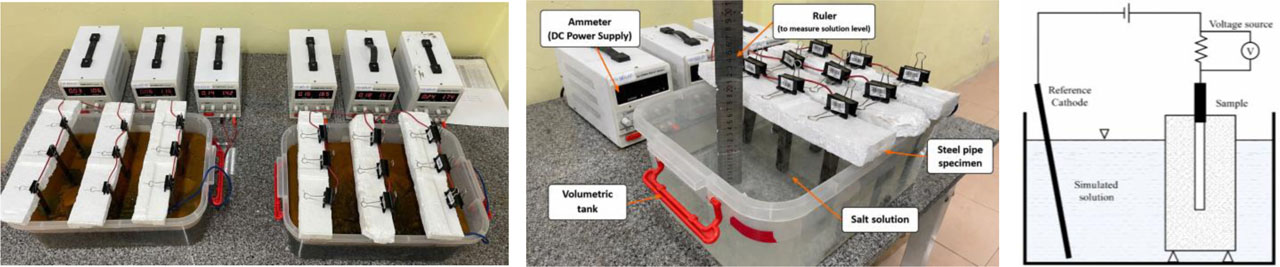
Figure 1:
Accelerated corrosion test setup for the SKK490 steel coupons under simulated Vietnamese marine conditions (Nguyen & Le Trung, 2025)
The test rig shown in Figure 1 comprised a DC power supply, an ammeter, a tank containing the simulated seawater, the partially immersed steel coupon, an Ag/AgCl reference electrode, and a stainless-steel counter electrode. An immersion depth of 100 mm provided a controlled exposed area throughout the test.
The applied current was calculated following ASTM G102 from the target accelerated corrosion rate, exposed area, steel density, and equivalent weight of iron. The corrosion rate is related to the corrosion current density by:
The total applied current was then obtained from:
Where:CR - the expected corrosion rate,
K1 - the constant value used in Faraday equation,
icor - the corrosion current density,
ρ - the material density,
EW - the equivalent weight of the material, calculated as , where W is the atomic weight of the material and n is its valence.
The resulting current for the coupon geometry was approximately 160 mA. The exposure durations used below follow the calibration reported for the original test program (Nguyen & Le Trung, 2025); they are equivalent durations, not direct observations from natural marine exposure.
The laboratory durations were 72, 120, 240, 320, 480, 800, 1200, and 1600 h, corresponding to the equivalent exposure durations of 4.5, 7.5, 15, 20, 30, 50, 75, and 100 years defined in the original test program. Thirty replicate coupons were tested at the first three durations, whereas three coupons were tested at each longer duration. After exposure, the coupons were removed, corrosion products were cleaned according to the experimental procedure, and the remaining mass was measured. Table 5 reports the laboratory duration, adopted equivalent exposure duration, number of specimens, and applied current.
Table 5:
Laboratory test duration and adopted equivalent exposure duration (Nguyen & Le Trung, 2025)
| Test stage | Test duration [hours] | Equivalent exposure duration [years] | Number of specimens | Applied current [mA] |
|---|---|---|---|---|
| 01 | 72 | 4.5 | 30 | 160 |
| 02 | 120 | 7.5 | 30 | |
| 03 | 240 | 15 | 30 | |
| 04 | 320 | 20 | 3 | |
| 05 | 480 | 30 | 3 | |
| 06 | 800 | 50 | 3 | |
| 07 | 1200 | 75 | 3 | |
| 08 | 1600 | 100 | 3 |
The accelerated test was intended to reproduce cumulative chloride-induced mass loss, not the full corrosion morphology of an offshore structure. It does not reproduce wave action, tidal wet-dry cycling, biofouling, variations in dissolved oxygen, or local hydrodynamic effects. Impressed-current testing is nevertheless a practical source of degradation data when long natural-exposure records are unavailable (Melchers, 2003a, 2003b; Wei et al., 2024).
The specimens are material coupons, not geometrically scaled pipe piles or offshore structures. Coupon size can affect current-density distribution, oxygen transport, pitting, hydrodynamic action, and corrosion-product development. Normalizing the response by mass reduces dependence on specimen mass but does not remove these effects. The results should therefore be interpreted as average coupon-level degradation under controlled accelerated conditions, not as direct estimates of full-scale wall-thickness loss.
The NGBM predicts cumulative corrosion mass loss only. The initial mechanical properties in Table 2 are provided to characterize the steel, but the model does not predict changes in yield strength, tensile strength, ductility, or residual structural capacity. Such assessment would require post-corrosion mechanical testing and a separate relationship between corrosion morphology, section loss, and mechanical performance.
Each experimental observation consists of a pair (t, c(t)), where t denotes the equivalent exposure time (year) and c(t) represents the measured corrosion mass loss ratio (%). Because only half of the specimen length was immersed in the solution, the corrosion mass-loss ratio was normalized by the initial mass of the immersed part, approximated as (m0/2), as follows:
Where:m0 - the initial specimen mass,
m(t) - the remaining specimen mass after exposure duration t.
The raw measurements were screened and summarized before model calibration to reduce the influence of experimental scatter. The NGBM was fitted to the representative values up to 30 years of equivalent exposure and then extrapolated to 100 years. The later experimental means were used only to assess the forecast.
Long-duration corrosion records are commonly incomplete because multi-decade exposure tests are expensive and slow. With only a few observations, flexible machine-learning models are prone to overfitting and unstable extrapolation. Grey-system methods were developed for small samples and incomplete information and are therefore examined here as an alternative (Julong, 1989).
The forecasting problem is thus defined as long-range extrapolation from a small, irregularly spaced calibration set. The evaluation focuses on numerical stability, physical admissibility, and uncertainty beyond the calibration interval.
2.2. Nonlinear Grey Bernoulli Model (NGBM)
The Nonlinear Grey Bernoulli Model (NGBM) is used to forecast corrosion mass loss from a small and irregularly sampled dataset. Grey System Theory is designed for systems with incomplete information and limited observations (Liu & Forrest, 2010). The Bernoulli exponent gives NGBM more flexibility than a fixed-form empirical regression when representing curvature in the degradation history.
For corrosion mass loss, an acceptable forecast must remain nonnegative, increase cumulatively, and stay below 100%. Parameter identification was therefore combined with numerical screening and these admissibility conditions.
The nonlinear grey Bernoulli differential equation is expressed as:
Where:x(1)(t) - the accumulated corrosion evolution sequence,
a - the linear development coefficient, b is the nonlinear forcing coefficient,
n - the nonlinear grey exponent controlling the evolution behavior of the degradation process.
The exponent n controls the curvature of the response. Values below unity can produce a transition from faster early growth to slower long-term accumulation, which is compatible with the progressive influence of corrosion products and transport limitations. In this study, however, n is treated as a phenomenological parameter rather than a direct measure of a single corrosion mechanism.
The analytical solution of the NGBM formulation can be written as:
Where:x(1)(1) - the initial accumulated corrosion state.
For the non-equidistant accumulated sequence used here, the original corrosion series is recovered by the corresponding inverse accumulated generation operation (IAGO) (Shen et al., 2016):
Unconstrained NGBM extrapolation can become unstable, especially when the exponent approaches a singular region. Sparse calibration data may then yield parameter sets that fit the observations but produce negative, non-monotonic, complex, or rapidly diverging forecasts.
The parameter search therefore rejects undefined or complex responses, exponential overflow, negative values, non-monotonic cumulative loss, and forecasts outside the 0–100% range. These checks are applied over the full prediction horizon, not only at the calibration points.
The admissible solution must satisfy three conditions: nonnegative mass loss, monotonic cumulative growth, and a finite upper bound. These are constraints on the reported degradation variable and do not imply that the instantaneous corrosion rate is constant or monotonic.
The resulting procedure retains the small-sample structure of NGBM while limiting implausible long-range behaviour and providing an uncertainty range for the forecast.
2.3. Implementation Procedure of the NGBM-Based Forecasting Approach
The analysis was carried out in six stages: statistical preprocessing, construction of the original sequence, non-equidistant accumulated generation, parameter identification, constrained extrapolation, and parametric-bootstrap uncertainty analysis.
Step 1. Statistical Preprocessing of the Corrosion Dataset
Before calibration, the replicate measurements were screened for outliers and summarized to obtain a stable representative sequence.
First, abnormal corrosion observations are removed using the interquartile range (IQR) criterion:
Where:Q1 and Q3 denote the first and third quartiles of the corrosion observations, respectively, and IQR = Q3 − Q1.
After outlier screening, the representative corrosion value at each exposure duration is obtained using the trimmed mean:
Where:x(i) - the ordered corrosion observation
n - the total number of observations
r - the number of values removed from each tail of the dataset
The final input sequence for the NGBM model is constructed as:
Where each term x(0)(k) corresponds to the representative corrosion mass loss ratio at the k-th exposure duration.
Standard deviation (SD) and coefficient of variation (COV) describe the spread among replicate measurements. The same SD values were used later to generate the parametric-bootstrap samples.
Step 2. Construction of the Original Corrosion Sequence
The experimental corrosion dataset is organized into the original discrete corrosion sequence:
For out-of-sample assessment, the representative observations at 4.5, 7.5, 15, 20, and 30 years were used for parameter calibration, while the observations at 50, 75, and 100 years were withheld from calibration and used only for comparison with the forecasts. The first observation was retained as the fixed initial grey state. This split tests whether the model can extrapolate a stable long-term trajectory from sparse early- and medium-duration observations.
Step 3. Accumulated Generation Operation (AGO)
To reduce stochastic fluctuation and improve sequence regularity, the accumulated generation operation is applied to the original corrosion sequence before grey differential modelling (Chen et al., 2008; Shen et al., 2016):
For the unequal exposure intervals in this dataset, accumulation is weighted by the elapsed time between successive observations:
Where:Δtk - the interval between consecutive exposure durations.
Equation (6) is the corresponding interval-normalized inverse, so accumulation and reconstruction remain consistent for unequal time steps (Shen et al., 2016; Xiao & Peng, 2011).
The neighbouring mean sequence is subsequently constructed as:
AGO converts the short, unevenly spaced series into a smoother accumulated sequence for parameter identification. This reduces the influence of local fluctuations without adding new observations.
Step 4. Parameter Optimization and Numerical Stabilization
The parameters a, b, and n were identified by constrained nonlinear minimization of a combined Root Mean Square Error (RMSE) and Mean Absolute Percentage Error (MAPE) objective over the calibration set (Chen, 2008; Lu et al., 2016):
The weights w1 and w2 balance absolute and relative error. Equal weights were used in the baseline calculation.
The RMSE and MAPE are defined as:
The search was bounded and used the combined RMSE-MAPE objective. A candidate was discarded if the analytical response was undefined or complex, overflowed numerically, became negative or non-monotonic, or exceeded the 0–100% physical range. Special attention was paid to values near n = 1, where the analytical expression is highly sensitive. These rules describe the calculation in a software-independent form.
Step 5. Constrained Long-Term Forecasting
The accepted parameter set was then used to extrapolate corrosion mass loss to 100 years, with particular attention to the interval beyond the 30-year calibration boundary.
To maintain physically meaningful corrosion behaviour, several constraints are incorporated into the forecasting process. The predicted corrosion mass loss is constrained below the physical upper limit:
Monotonic corrosion growth is additionally enforced through:
reflecting the irreversible and cumulative nature of marine corrosion degradation.These constraints apply to cumulative mass loss: material already lost cannot be recovered, and the total loss cannot exceed the initial mass. They do not require a constant or monotonic corrosion rate. Wet-dry cycling, rust cracking or spalling, biofouling, oxygen availability, and other environmental changes may alter the rate or create separate regimes. Where such changes are supported by data, a piecewise or regime-switching model would be more appropriate.
Step 6. Bootstrap Uncertainty Analysis
To quantify forecasting uncertainty under sparse-data conditions, a parametric bootstrap was applied to the calibration observations. Synthetic corrosion values were generated by adding independent Gaussian perturbations with standard deviations equal to the experimentally reported values at the corresponding exposure durations. The initial grey state was preserved to avoid an artificial translation of the complete forecast trajectory.
A total of 300 bootstrap realizations were evaluated. For each synthetic dataset, the NGBM parameters were re-identified using the same numerical-stability and physical-admissibility criteria as in the deterministic calibration. The ensemble mean was reported together with the 2.5th and 97.5th percentiles, which define a 95% bootstrap uncertainty interval for the forecast trajectory.
The interval represents uncertainty propagated from replicate dispersion and parameter identification under the adopted Gaussian perturbation model. It does not include every source of variability in natural marine exposure and should not be read as a universal confidence interval.
3. Results and Discussion
3.1. Statistical Characteristics of the Experimental Corrosion Dataset
Table 6 summarizes the processed calibration data. All mass-loss quantities are reported in percent. Trimmed means were calculated after IQR screening; SD and COV describe replicate dispersion, while the 95% intervals refer to uncertainty in the representative means.
Figure 2 plots the trimmed means and their 95% intervals. The measured SD values, rather than the plotted intervals, were used to generate perturbations in the parametric bootstrap.
Table 6:
Statistical summary of pre-processed corrosion data
| Years | Trimmed Mean [%] | SD [%] | COV [%] | 95% CI Lower [%] | 95% CI Upper [%] |
|---|---|---|---|---|---|
| 4.5 | 3.78 | 0.26 | 6.9933 | 3.68 | 3.88 |
| 7.5 | 5.77 | 0.39 | 6.7339 | 5.62 | 5.91 |
| 15 | 14.18 | 1.04 | 7.3116 | 13.80 | 14.57 |
| 20 | 15.72 | 0.17 | 1.1055 | 15.29 | 16.15 |
| 30 | 22.21 | 0.17 | 0.7745 | 21.78 | 22.64 |
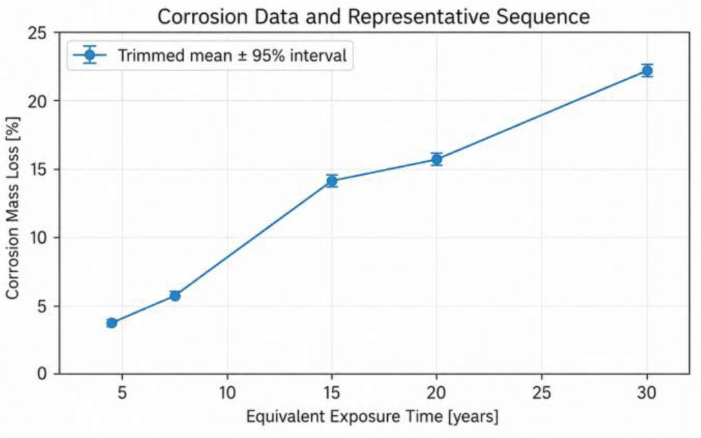
Figure 2:
Experimental corrosion mass-loss ratio with trimmed mean and 95% confidence interval
Figure 3 presents the measured mass loss from 4.5 to 100 years of equivalent exposure. The observation times are unevenly spaced and only a few representative points are available, which is typical of long-duration accelerated corrosion programs.
Cumulative mass loss increases with exposure, but its rate changes over time. The response is relatively rapid at early ages and slower over part of the later record. Corrosion-product formation may contribute to this pattern by restricting oxygen and chloride transport, although the present measurements cannot identify a single governing mechanism.
This changing curvature makes extrapolation difficult. A model fitted only to early observations may overpredict later loss, whereas an unconstrained nonlinear model may fit the calibration range and still diverge beyond it. Unequal time spacing and experimental scatter add further uncertainty.
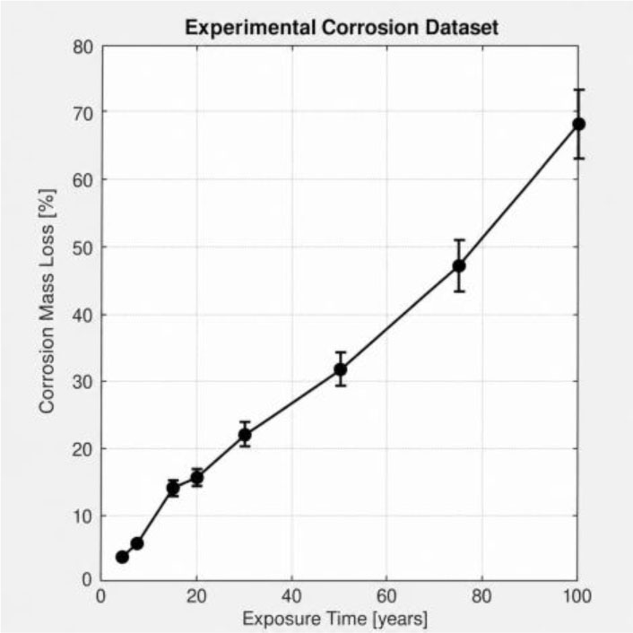
Figure 3:
Experimental corrosion mass-loss ratio over equivalent exposure time
3.2. AGO Transformation and Sequence Regularization
Figure 4 shows the sequence after the non-equidistant accumulated generation operation (AGO) used for unequal observation intervals (Shen et al., 2016; Xiao & Peng, 2011). The transformation produces a smoother sequence for parameter identification.
The vertical axis in Figure 4 is the accumulated AGO sequence, not corrosion mass loss in percent. Its larger numerical values arise from the transformation and should not be interpreted as direct material loss.
This regularized sequence is less sensitive to local fluctuations and unequal time intervals than the original observations, which improves numerical identification of the grey differential equation.
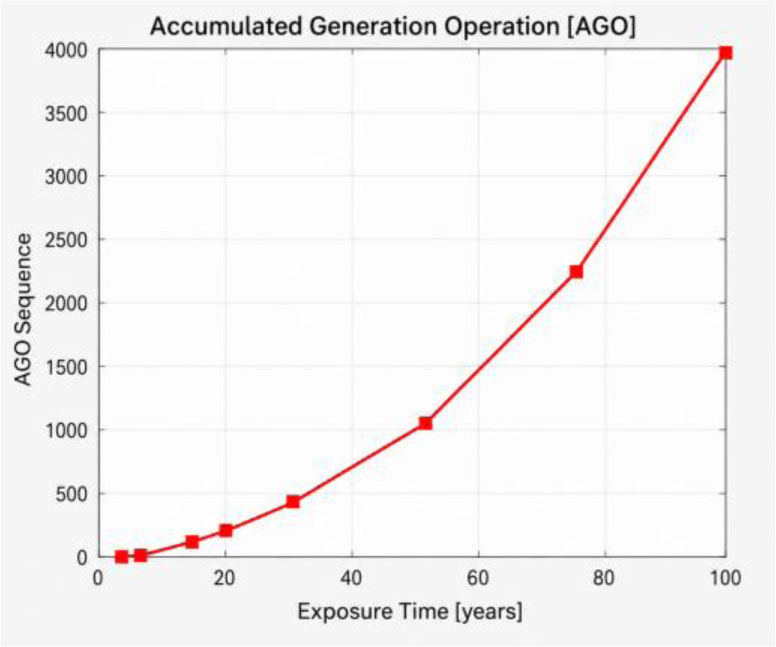
Figure 4:
Smoothed corrosion sequence generated by the non-equidistant accumulated generation operation (AGO)
3.3. Numerical Instability and Constraint Effects on Long-Term Forecasting
Figure 5 is a sensitivity study, not a set of equally acceptable forecasts. The plotted curves were generated for a prescribed grid of n values to show how strongly the exponent affects long-term behaviour. The optimized value, n = 0.419, was obtained separately from the constrained calibration and is used for the deterministic forecast.
Mathematically, this instability is associated with the structural exponent term:
Small values of n give low, strongly decelerating trajectories, whereas values near the singular region can produce rapid or unstable growth. Minimization of the combined RMSE-MAPE objective subject to the admissibility checks gave n = 0.419.
The fitted value n = 0.419 is below unity and gives a sub-linear accumulated response. It may reflect the combined effects of corrosion-product formation, transport resistance, and evolving electrochemical conditions, but the present dataset does not allow n to be assigned to any one mechanism. It is therefore treated as a phenomenological model parameter.
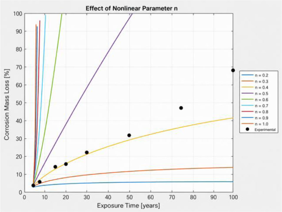
Figure 5:
Sensitivity of the long-term NGBM response to prescribed values of the nonlinear exponent n; the optimized value n = 0.419 is reported separately and used for forecasting
3.4. Bootstrap Uncertainty Analysis of Long-Term Corrosion Forecasting
Figure 6 shows the parametric-bootstrap forecast. Three hundred synthetic calibration datasets were generated by adding independent Gaussian perturbations with SD values equal to the measured replicate dispersion at each exposure duration; the initial grey state was kept fixed. The NGBM was re-identified for every realization using the same admissibility checks. Faint lines denote individual forecasts, the solid line is their mean, and the shaded band spans the 2.5th–97.5th percentiles.
The interval is narrow near the calibration data and widens after 30 years as measurement dispersion and parameter uncertainty propagate into the extrapolation. It is conditional on the Gaussian perturbation model and is reported as a bootstrap uncertainty interval, not as a confidence band applicable to all marine environments.
Wet-dry cycling, biofouling, local pitting, and variations in dissolved oxygen are not represented explicitly. The interval therefore covers uncertainty within the present statistical model, not every source of field variability.
For this dataset, all 300 bootstrap realizations were completed within a few seconds on a standard desktop computer. The calculation is therefore modest in cost, although execution time will depend on the implementation and hardware.
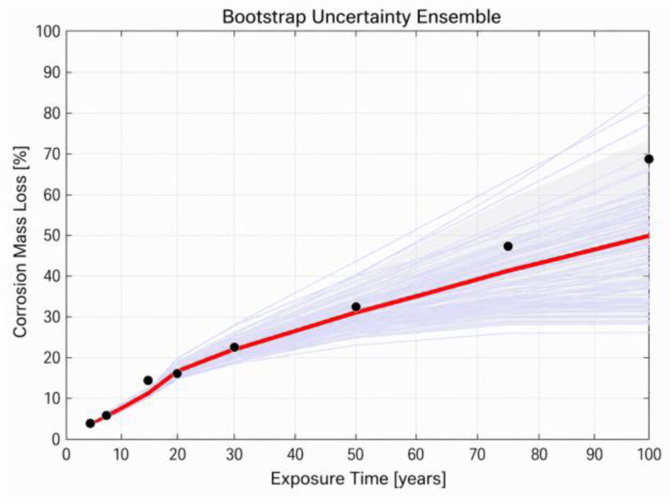
Figure 6:
Parametric-bootstrap ensemble, mean NGBM forecast, and 95% uncertainty interval
3.5. Comparison with Weibull and Power-Law Benchmark Models
Figure 7 compares the constrained NGBM with Weibull and power-law models calibrated on the same observations. The two empirical models are included as benchmarks rather than as physically constrained alternatives.
Beyond the 30-year calibration limit, both benchmark curves rise more steeply than the NGBM trajectory. At 100 years, the Weibull and power-law forecasts are approximately 78% and 76%, respectively, whereas the deterministic NGBM forecast is about 50%. The experimental means at 75 and 100 years lie closer to the empirical curves. Thus, NGBM does not give the smallest pointwise error at every withheld observation; its advantage in this comparison is controlled, bounded extrapolation together with an uncertainty interval.
The deterministic NGBM underestimates the means at 75 and 100 years, but those observations fall within the bootstrap interval. This finding illustrates the uncertainty created by the short calibration series; it does not establish that NGBM is generally more accurate than the benchmark models. Conversely, the good agreement of the empirical curves at some late points does not guarantee stable continuation beyond the observed range.
The comparison highlights a practical trade-off: the empirical benchmarks match some late observations more closely, while NGBM provides an admissibility-screened trajectory and an explicit estimate of extrapolation uncertainty.
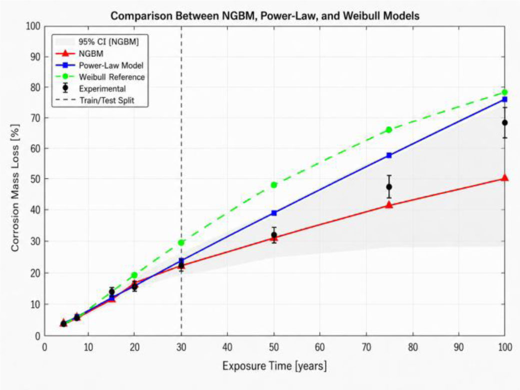
Figure 7:
Comparison of the NGBM forecast and 95% uncertainty interval with experimental observations and the calibrated Weibull and power-law benchmarks
4. Conclusions
This study developed a constrained NGBM for cumulative corrosion mass loss in SKK490 steel coupons using a short, irregularly spaced dataset. Observations up to 30 years of equivalent exposure were used for calibration, and those at 50–100 years were retained for out-of-sample comparison. Non-equidistant accumulation, admissibility screening, and a parametric bootstrap were used to obtain nonnegative, monotonic, and bounded forecasts.
The optimized exponent was n = 0.419. It describes the curvature of the fitted response but should not be interpreted as a measured corrosion-mechanism constant without further experimental evidence.
At 100 years, the Weibull and power-law benchmarks predicted about 78% and 76% mass loss, respectively, while the deterministic NGBM predicted about 50%. The benchmark models were closer to some of the withheld observations. The value of the constrained NGBM in this study is therefore not uniformly lower pointwise error, but a bounded extrapolation accompanied by a quantified uncertainty range.
The 300-realization bootstrap interval widened after the calibration boundary and included the late observations. This interval is conditional on the assumed Gaussian perturbations and the limited calibration dataset.
The conclusions are limited to one impressed-current program, one steel grade, and the adopted equivalent-exposure scale. The coupons are not scaled pipe specimens, and the model does not predict pitting, residual wall thickness, changes in yield strength, or structural capacity. Application to design or maintenance decisions will require validation against natural marine exposure, larger specimens, other steels and exposure zones, and post-corrosion mechanical tests. If future datasets show distinct corrosion regimes, piecewise or regime-switching formulations should also be considered.
Acknowledgements
The authors acknowledge the laboratory staff and research collaborators who supported the accelerated corrosion testing program.
Notes
[1] Contributed by Author Contributions
T.T.T.N. conceived and designed the study, developed the research framework, and contributed to manuscript preparation. T.H.L. conducted the accelerated corrosion experiments and contributed to data collection and interpretation. N.T.T. contributed to statistical analysis and model implementation. Q.T.N. contributed to data interpretation and manuscript review. All authors critically reviewed and approved the final version of the manuscript and agreed to be accountable for all aspects of the work.