

1. Introduction
With the increasing service life of tunnels, various structural defects gradually emerge, among which lining cavities have become a critical issue affecting structural safety and durability (Chen et al, 2024). These cavities are typically caused by construction deficiencies, adverse geological conditions (Basirat, 2025), and environmental factors (Gu et al., 2026). Their presence can significantly reduce the stiffness and load-bearing capacity of the lining, potentially leading to problems such as water seepage, crack propagation, and even structural failure. Therefore, the timely and accurate detection of cavity defects is essential for effective tunnel health monitoring and maintenance.
Conventional methods for detecting cavities in tunnel linings include ground-penetrating radar (GPR) and the impact-echo method, each with inherent advantages and limitations. GPR detects subsurface anomalies by analysing electromagnetic wave reflections and is effective for identifying relatively large defects (Chen et al., 2025; Alsharqawi et al., 2022). However, its performance is significantly affected in moist or water-rich environments due to severe signal attenuation. The impact-echo method evaluates structural integrity through stress wave reflections generated by mechanical impacts. Nevertheless, it requires physical contact with the structure, which may cause surface damage, and its point-by-point operation leads to low inspection efficiency, making it unsuitable for large-scale applications (Yang et al., 2025). To overcome these limitations, recent studies have explored advanced structural health monitoring techniques, including flexible strain sensors based on graphene materials (Weng et al., 2025; Wang and Zhang, 2022), optical fibre sensing technologies (Wang et al., 2019) and data-driven prediction or assessment methods (Meng et al., 2025; Xiong et al., 2025). While these methods offer high sensitivity and long-term monitoring capabilities, they generally rely on contact installation and therefore lack the ability to perform remote inspections.
In recent years, non-contact acoustic inspection (NCAI) technologies have attracted increasing research attention due to their efficiency and non-destructive nature, and they have been widely applied in the field of nondestructive testing (NDT) (Gulino et al., 2022; Tham et al., 2024; Wandowski et al., 2023; Datta et al., 2023; Sugimoto et al., 2024). For example, Alkhateeb et al. (2022) investigated the feasibility of detecting and localizing corrosion damage using acoustic emission (AE). Sampath et al. (2025) proposed a non-contact, laser-excited acoustic shearography technique for rapid, full-field imaging of micro-cracks. Xiao and Yu (2021) introduced air-coupled transducers for non-contact AE signal detection on composite structures.
LDV has emerged as a powerful tool in structural health monitoring due to its high precision, non-contact measurement capability, and sensitivity to minute vibrations (Li et al., 2022; Fu et al., 2025). Based on the Doppler effect, LDV technology captures frequency shifts in reflected laser light to measure surface vibrations (Seydipour and Rezaei, 2025). Compared to traditional contact-based sensors, LDV technology avoids physical contact, thereby eliminating the risk of structural damage (Darwish et al., 2025). It has been widely applied in civil engineering (Martínez et al., 2026; Zhang et al., 2025) and agriculture (Landahl and Terry, 2020).
Despite these advancements, a significant research gap remains in the quantitative characterization of subsurface cavities in thick concrete structures using LDV. Most existing LDV-based non-destructive testing (NDT) methods primarily focus on the qualitative identification of surface-level defects or thin-walled structures. There is a lack of systematic research that explicitly formulates the relationship between the geometric parameters of deep concrete cavities and their multi-modal resonance responses – specifically the interaction between bending resonance and thickness vibration – under remote acoustic excitation. To address this research gap, the present study introduces a high-precision diagnostic criterion based on the simultaneous identification of bending resonance and thickness vibration. We establish and experimentally validate a quantitative mapping between cavity geometric parameters—specifically diameter and depth – and corresponding resonance frequency shifts. Furthermore, systematic evaluations demonstrate that while vibration amplitude attenuates significantly with distance, the resonance frequency remains an invariant and robust indicator for remote structural health monitoring at ranges up to 10 meters. Collectively, these findings provide a rigorous theoretical and technical foundation for advancing from qualitative “presence detection” to quantitative “defect assessment” in concrete infrastructures.
2. Principle of Remote Detection of Cavities in Concrete
2.1. Analysis of the Principle of Laser Doppler Detection
LDV is based on the optical Doppler effect, in which the frequency of light reflected from a moving object differs from that of the incident beam. This frequency shift contains information about the vibration characteristics of the object and is referred to as the optical Doppler shift. Since both the light source and photo detector (PD) remain stationary, and the positions of the light source, moving particles, and PD as well as the directions of light propagation and particle motion are known, the velocity of the particle can be determined using the principle of the Doppler effect of light.
A laser beam with wavelength λ is directed onto the surface of a vibrating object in the LDV system. In a heterodyne interferometer, the beam is split by Beam Splitter (BS) 1 into a measurement beam and a reference beam. The measurement beam strikes a specific point on the vibrating object, and the reflected light returns to BS 2, where it interferes with the reference beam at BS 3. The working principle of LDV technology is illustrated in Figure 1. If the object is vibrating, the interference process generates fluctuations in the intensity of the light signal. When the object moves by half a wavelength, the detector converts the resulting signal into voltage fluctuations. The frequency of the reflected laser light changes, producing a Doppler shift fD. This sinusoidal Doppler shift fD is directly proportional to the velocity v of the object, as shown in Equation (1):
Where:fD - the Doppler frequency shift (Hz),
v - the instantaneous vibration velocity of the target surface (m/s),
λ - the wavelength of the incident laser beam (m).
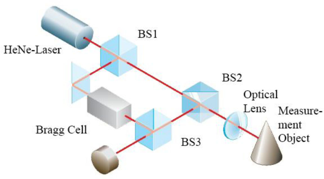
Figure 1:
Schematic of the LDV working principle
By measuring the Doppler frequency shift fD, the velocity v of the moving object can be calculated. By decoding the output signal of the LDV using a controller, information about the vibration characteristics of the target, such as motion frequency and amplitude, can be obtained.
2.2. Angle Dependence
As shown in Figure 2, the sound pressure distribution p(x) acts on the defect area at an incident angle θ, where λ is the wavelength of the acoustic wave. The function u(x) represents the result obtained by projecting the normal mode amplitude of the defect surface onto the x-axis. According to the reciprocity principle, the vibration amplitude of the defect area induced by the acoustic excitation can be obtained through the cross-correlation between the modal amplitude u(x) and the sound pressure distribution p(x). When the incident acoustic wave is a sinusoidal wave, this relationship is equivalent to a Fourier transform.
In acoustic wave propagation, the sound pressure distribution is typically closely related to the wave propagation direction, the propagation angle, and the properties of the medium. Assuming that the angle between the propagation direction of the acoustic wave and the normal to the defect surface is θ, the sound pressure distribution p(x) can be expressed by Equation (2):
Where:p0 - the initial sound pressure amplitude,
i - the imaginary unit used in the complex representation of harmonic waves,
k - the number of wave cycles per unit length, calculated by k = 2π/λ,
x - the spatial position, measured along the direction of the defect surface,
θ - the angle between the direction of acoustic wave, propagation and the surface normal,
ω - the angular frequency.
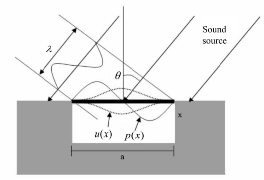
Figure 2:
Schematic of acoustic incident angle θ and resulting vibration amplitude u(x)
Acoustic waves are typically represented as sinusoidal waves, but due to the incident angle θ, the propagation direction changes, resulting in a spatial distribution that becomes a complex function of x.
The vibration amplitude on the surface of a defect is generally determined by the surface morphology of the defect and the applied acoustic excitation. This amplitude can be expressed as a function u(x), which is typically associated with the geometric shape and material properties of the defect surface. Assuming the deformation along the x-direction on the defect surface is u(x), it can be described by Equation (3):
Where:ψ(k) - the vibration mode of the defect surface corresponding to the wave number κ.
This form describes the vibration amplitude using a Fourier transform, indicating that the vibration of the defect surface can be represented as a superposition of multiple vibration modes at different frequencies. According to the reciprocity principle, the relationship between the vibration of the defect surface under acoustic excitation u(x) and the sound pressure distribution p(x) can be described by cross-correlation. Specifically, this relationship can be expressed by Equation (4):
Where:R(x, x′) - a reciprocity-based response function describing propagation from x′ to x.
In the Fourier domain, the reciprocity principle can be expressed by Equation (5):
Where:- the Fourier transform of the vibration amplitude,
- the Fourier transform of the response function,
- the Fourier transform of the sound pressure distribution.
2.3. Thickness Vibration and Bending Resonance
Under external excitation, when longitudinal waves are applied to the surface of concrete, they exhibit strong directivity along the surface normal. Additionally, due to their higher wave velocity compared to other stress waves, longitudinal waves can induce larger particle displacements. Therefore, this study primarily employs longitudinal waves to detect internal cavities in concrete.
Consider an infinite concrete slab with a thickness of H, composed of a linear elastic, isotropic, and homogeneous medium. It is assumed that the longitudinal wave generated by acoustic excitation can be idealized as a spherical wave, as illustrated in Figure 3(a), where the p-wave represents the longitudinal wave induced by laser excitation. In the figure, Z1 and Z2 denote the wave impedances of the material inside the slab and the surrounding medium, respectively. When the longitudinal wave reaches the back surface of the slab, the change in wave impedance caused by the difference in media leads to reflection and mode conversion. Specifically, the 2p-wave represents the longitudinal wave reflected from the back surface, while the ps-wave refers to the shear wave generated through mode conversion at the back surface.
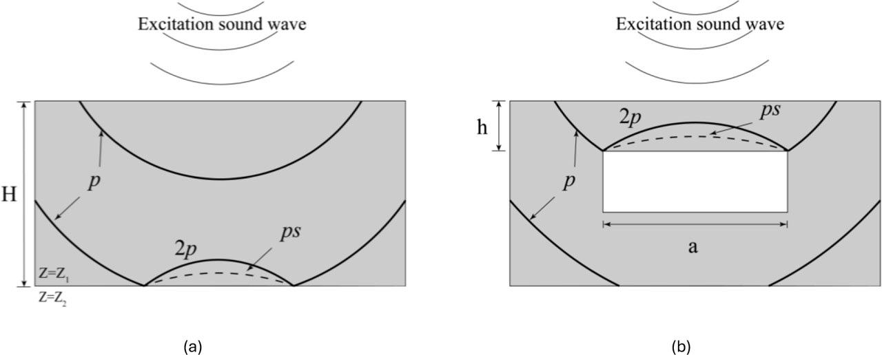
Figure 3:
Acoustic wave reflection and mode conversion at (a) the specimen backwall and (b) an internal cavity interface
When the acoustic wave reflects between the surface and the back wall of the slab, a longitudinal wave resonance is formed, which is referred to as thickness vibration. The frequency of the thickness vibration can be expressed by Equation (6):
Where:CL - the velocity of the longitudinal wave, typically measured at the material surface,
H - the thickness of the slab,
κ - the boundary condition coefficient.
When Z1 > Z2, for example, in the case of a solid/air interface at the back surface, the parameter κ = 2. In this situation, the back surface can be regarded as a free boundary, where compression waves are converted into tensile waves. In Figure 3(a), the p-wave incident on the back surface is a compression wave, while the 2p-wave reflected from the back surface is a tensile wave. When Z1 < Z2, the back surface can be considered a solid/rigid-solid interface. The longitudinal wave reflection at this interface is characteristic of a steel-wall reflection. The back surface can then be treated as a fixed boundary, and no conversion between compression and tensile waves occurs. In this case, the parameter κ = 4.
Studies have shown that when the slab in Figure 3(a) is a concrete slab with finite dimensions, the longitudinal wave velocity inside the slab is approximately 95% of the surface-measured longitudinal wave velocity CL. This is generally attributed to multiple reflections of the longitudinal wave within the concrete. Therefore, the thickness resonance frequency of the concrete slab fH is given by:
Equation (7) is the calculation formula commonly used in industry for measuring the thickness of concrete slabs using the impact-echo method, where κ is typically taken as 2. It is evident that the thickness resonance frequency in Equation (7) is obtained by dividing the longitudinal wave velocity in concrete by the travel path. The propagation time TH of the longitudinal wave reflected from the back surface of the slab is given by Equation (8):
In practice, the longitudinal wave resonance frequency generated between a defect located at a depth h within the concrete and the surface can be expressed as:
As shown in Equation (9), when the wave velocity CL remains constant, the longitudinal resonance frequency of a defect depends solely on its location.
The case where a cavity exists at a depth h within the concrete slab is illustrated in Figure 3(b), with the cavity having a diameter a. The wave impedance coefficients of air and concrete are listed in Table 1.
Table 1:
Wave impedance coefficients of air and concrete
| Material | Wave impedance coefficients |
|---|---|
| Air | 0.4 |
| Concrete | 7×10⁶∼12×106 |
Under perpendicular incidence of a longitudinal wave, the reflection coefficient F of the reflected wave is given by:
According to the data in Table 1, the wave impedance of air is nearly 0. Based on the calculation from Equation (10), when a stress wave encounters the interface between concrete and air, the reflection coefficient is nearly 1. As a result, the longitudinal wave incident on the cavity interface is almost completely reflected. The longitudinal wave undergoes repeated reflections between the concrete surface and the cavity, forming longitudinal wave resonance. In this case, the thickness vibration frequency of the cavity can be calculated using Equation (9).
Studies have shown that the size a and depth h of cavities within concrete have a significant effect on the propagation characteristics of acoustic waves. When a < 0.3h, longitudinal waves diffract and reflect from the back wall of the cavity, resulting in an increased propagation path and a frequency shift toward the lower range. When 0.3h ≤ a ≤ 1.5h, the echo contains components from both cavity-reflected and diffracted waves. In this case, the frequency spectrum shows both the reflection peak induced by the cavity defect and the thickness resonance frequency peak. Compared to the case without a cavity, the thickness resonance frequency also shifts to a lower frequency. When a > 1.5h, longitudinal waves are completely reflected at the cavity boundary. If the cavity is shallow and located just beneath the concrete surface, it reduces the flexural stiffness of the overlying concrete, leading to a decrease in structural stiffness.
Based on the above dynamic behaviour, the concrete response can be approximated as that of a simply supported plate. The first-order natural frequency of its bending vibration can be calculated using Equation (11):
Where:h - the depth of the cavity,
E - the Young's modulus of the concrete,
ρ - the density of the concrete,
a - the diameter of the cavity,
μ - Poisson’s ratio.
This equation indicates that the presence of a cavity affects the vibration characteristics and natural frequency of the concrete surface. When a cavity appears within the concrete tunnel lining, the concrete surface directly above the cavity exhibits bending vibration characteristics. In this case, resonance peaks associated with bending vibration will appear in the frequency spectrum. By observing the presence or absence of such resonance peaks, the existence of internal cavities within the concrete can be effectively identified.
According to research investigations, the area of cavities behind tunnel concrete linings is mostly in the range of 0.3m2 to 5m2, while the depth h typically ranges from 0.05m to 0.3m. Based on Equation (11), the first-order natural frequencies of cavities with areas from 0.1m2 to 5m2 and depths from 0.1m to 0.3m were calculated. The results are shown in Figure 4(a) illustrates the bending vibration frequencies of the concrete surface above cavities at different depths, while Figure 4(b) shows the relationship between cavity area and the bending vibration frequency of the overlying concrete. The black dashed lines represent the longitudinal resonance frequencies generated between defects at various depths and the surface. As shown in the Figure 4, when cavities exist within the concrete, the first-order natural frequency of bending vibration increases with cavity depth but decreases as the cavity area increases.
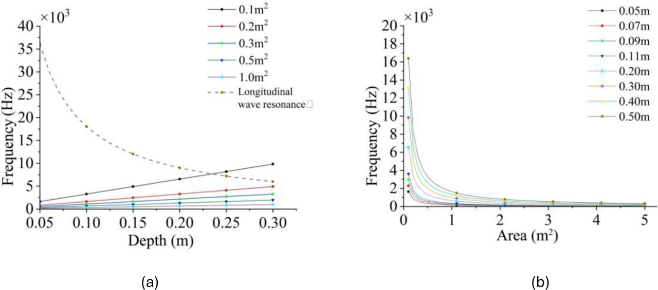
Figure 4:
Relationship among cavity area, depth, and bending vibration frequency: (a) Bending vibration frequency of concrete above cavities at different depths; (b) Relationship between cavity area and the bending vibration frequency of the concrete above
3. Preparation for Physical Experiment
This section describes the design of concrete specimens featuring diverse cavity dimensions and depths. Vibration was induced via both mechanical hammer impact and remote non-contact acoustic excitation. The acquired responses were analyzed to characterize vibration behaviors and establish correlations between cavity parameters and their natural frequencies.
3.1. Fabrication of Concrete Specimens
In this experiment, six concrete specimens were fabricated using C30 concrete. All specimens were cast with C30-grade concrete. The mix proportions of the concrete are shown in Table 2.
Table 2:
Mix proportion of C30 concrete (kg/m3)
| Materials | Cement | Water | Sand | Gravel | Water-Reducing Agent |
|---|---|---|---|---|---|
| Mix proportions | 350 | 175 | 690 | 1050 | 2.1 |
The dimensions of the six concrete specimens are listed in Table 3, with the thickness of the cavity section set uniformly at 100 mm. Figure 5 presents a schematic diagram of these specimens.
Table 3:
Working condition settings
| Dimensions (L×W×H) | Cavity diameter a [mm] | Depth from surface [h] | |
|---|---|---|---|
| Specimen 1 | 400×300×300 | 100 | 20 |
| Specimen 2 | 500×400×300 | 200 | 20 |
| Specimen 3 | 600×500×300 | 300 | 20 |
| Specimen 4 | 600×500×300 | 300 | 50 |
| Specimen 5 | 600×500×300 | 300 | 80 |
| Specimen 6 | 600×500×300 | No Cavity, Solid Specimen | |
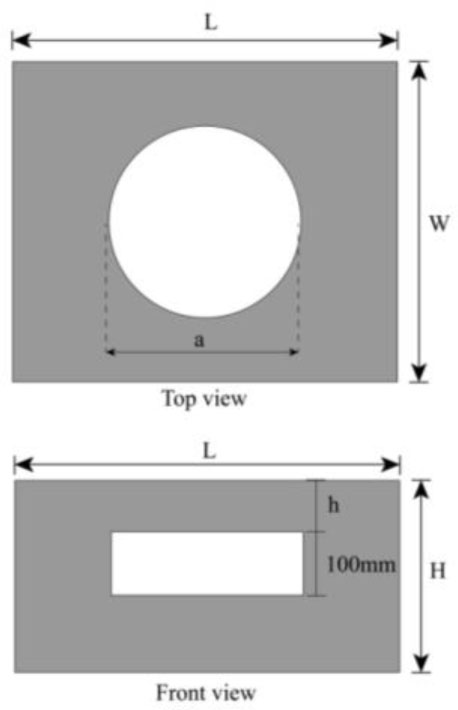
Figure 5:
Schematic diagram of the specimen
The casting process of concrete specimens with cavities is illustrated in Figure 6: template making, pouring of concrete, component processing, component maintenance.
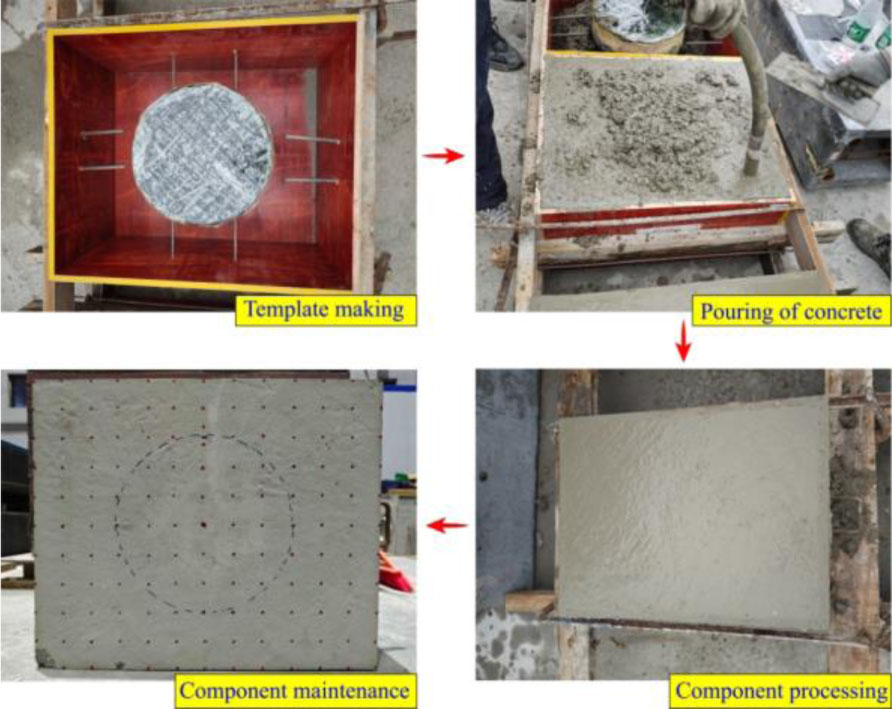
Figure 6:
Concrete specimen casting process
3.2. Testing Procedure
1). Experimental system
A schematic diagram of the testing equipment is shown in Figure 7. The experimental system primarily consists of a Laser Doppler Vibrometer and a directional acoustic excitation system. The LDV features a frequency bandwidth of 2.5MHz and a displacement resolution of 0.01nm, with a laser output power of 5mW. The directional acoustic source operates within a range of 0–10kHz, delivering a maximum sound pressure level (SPL) of 145dB (measured at 1m) and a peak power of 800W. During the tests, both the LDV and the excitation device were positioned at a horizontal distance of d=5m from the specimen and integrated via a laptop-based control interface. To ensure a high signal-to-noise ratio, the experimental environment was strictly managed to eliminate external acoustic interference.
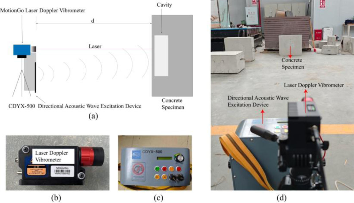
Figure 7:
Schematic diagram of test equipment layout: (a) LDV detection test diagram; (b) Laser doppler vibrometer; (c) Directional acoustic wave excitation device; (d) Layout diagram of on-site test equipment
2). Parameter settings of the directional acoustic wave excitation device
Figure 8 illustrates the acoustic waveform generated by the directional excitation system. A pulse duration of 3 ms was utilized—yielding an approximate bandwidth of 330 Hz—with a 50 ms interval between successive pulses. To ensure spectral coverage across the 1–6000 Hz range, a 200 Hz frequency modulation interval was implemented, effectively activating the target frequency band. The 50 ms pulse interval facilitates complete propagation over a 15-m distance (requiring ~43 ms), thereby precluding signal overlap. This configuration aligns with the acoustic round-trip period, ensuring high-fidelity signal acquisition while minimizing temporal interference. Furthermore, the excitation amplitude was optimized to ensure robust detection performance.
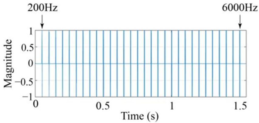
Figure 8:
Audio signal diagram of the acoustic excitation device
4. Comparative Testing under Hammer Excitation and Acoustic Excitation
4.1. Time-domain Signal Processing Method
Figure 9 depicts the spatial distribution of measurement points for Specimen 3, where vibration signals were acquired at locations 1–4. Two excitation modalities were implemented: mechanical hammer impact and remote acoustic excitation, representing contact-based and non-contact sources, respectively. The vibration responses were acquired using a Laser Doppler Vibrometer, followed by a comparative analysis of the excitation-dependent characteristics of the concrete structure.
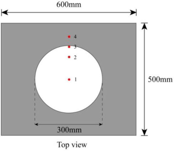
Figure 9:
Measurement point layout diagram
Figure 10 (a) illustrates the time-domain vibration response of a measurement point on Specimen 3 under acoustic excitation. Within the 1.5-s excitation window, three distinct wave packets are clearly discernible, reflecting the pulse sequence emitted by the directional acoustic system. However, the raw signals exhibit significant stochastic noise and broadband interference, resulting in complex spectral characteristics that mask the intrinsic structural vibration features.
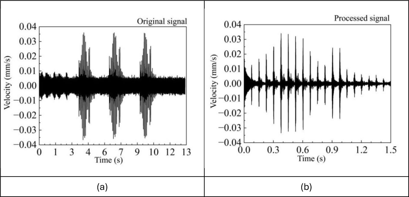
Figure 10:
Comparison of time-domain signals before and after processing: (a) Original signal; (b) Processed signal
Figure 10 (b) illustrates the time-domain vibration response after signal preprocessing. The raw vibration data, acquired at a high sampling rate of 312,500 Hz, were pre-processed using the MATLAB Signal Analyzer to ensure high fidelity in the frequency domain. To isolate the characteristic vibration components associated with internal cavities, a digital band-pass filter with a passband of 500–6,000 Hz was implemented. The filter was specifically configured with a steepness of 0.85 and a stopband attenuation of 60 dB to effectively suppress low-frequency environmental noise and high-frequency instrumentation interference. As shown in Figure 10(b), the noise level in the processed signal was substantially reduced, and key frequency features became clearly distinguishable, providing a stable and reliable basis for subsequent structural spectral analysis.
4.2. Time-frequency Spectrum Analysis at Different Measurement Points under Hammer Excitation
Figure 11 illustrates the vibration response characteristics at four measurement points under hammer impact. To ensure consistent excitation force, the hammer was released from a fixed height for each strike. The time-domain waveforms (a–d) and corresponding frequency spectra (e–h) reveal a prominent peak near 770 Hz at all locations, identifying the bending resonance frequency of the concrete slab overlying the cavity. Specifically, Point 1 exhibits the maximum velocity amplitude of 12.51 mm/s at 760 Hz, while Point 2 displays a comparable resonance frequency with a reduced amplitude of 5.79 mm/s. As the distance from the cavity center increases, the amplitudes at Points 3 and 4 attenuate significantly to 0.17 mm/s and 0.08 mm/s, respectively. Spectral analysis indicates that the 770 Hz peak amplitude decays monotonically as the distance from the cavity center increases, aligning with observations from acoustic excitation. This validates the spatial attenuation profile of the vibration response as it propagates radially from the cavity. This phenomenon demonstrates that the surface velocity field – measured via Laser Doppler Vibrometer – exhibits a radial spatial distribution, characterized by peak amplitude at the cavity center and progressive attenuation toward the periphery.
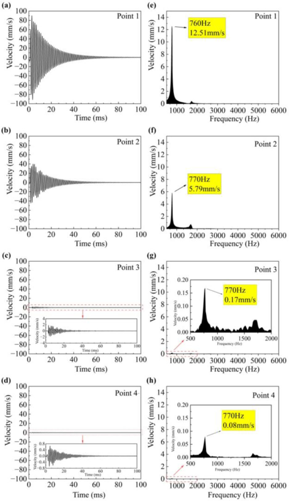
Figure 11:
Time-domain and frequency spectrum analysis of Specimen 3 at points 1–4 under impulsive hammer excitation
4.3. Time–frequency Spectrum Analysis at Different Measurement Points under Remote Acoustic Excitation
Figure 12 illustrates the vibration response characteristics at four locations under acoustic excitation. The time-domain waveforms (a–d) exhibit distinct vibrational patterns among the measurement locations. Spectral analysis (e–h) reveals two characteristic peaks at each location: a bending resonance at 821 Hz and a thickness vibration mode at 4809 Hz. The peak at 821 Hz, identified as the cavity-related bending mode, exhibits a systematic amplitude attenuation with increasing distance from the cavity center. Specifically, the velocity amplitudes captured by the Laser Doppler Vibrometer from 3.77×10⁻⁴ mm/s at Point 1 to 2.93×10⁻⁴ mm/s at Point 2, further declining to 1.19×10⁻⁴ mm/s at Point 3, before becoming negligible at Point 4. In contrast, the amplitude of the 4809 Hz thickness vibration remains relatively stable across all measurement points (2.00×10⁻⁴ to 2.43×10⁻⁴ mm/s). This stability arises because this mode is exclusively determined by the specimen thickness and wave velocity (Equation (7)). Notably, the Laser Doppler Vibrometer detected only the thickness mode at Point 4 (located in the solid region). This finding further confirms the exclusive correlation between the bending resonance and the presence of sub-surface cavities.
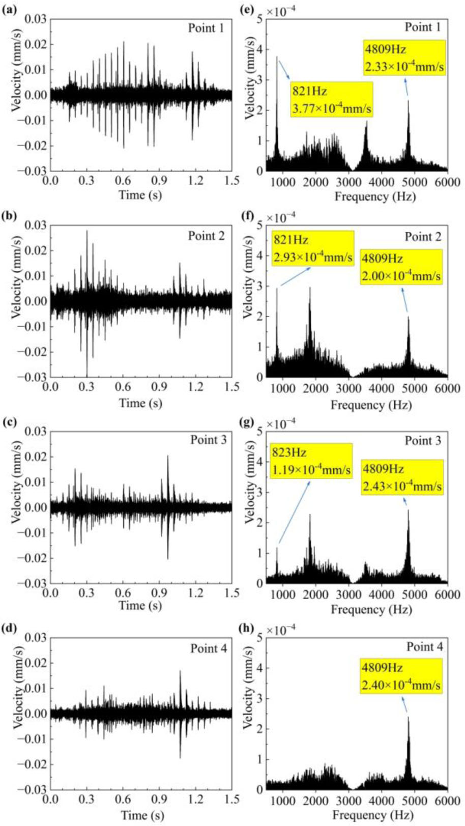
Figure 12:
Time-frequency spectrum analysis at different measurement points under remote acoustic excitation
Based on the time-domain and spectral analyses presented in Figure 12, it is evident that the vibration characteristics of the concrete cavities exhibit pronounced spatial locality, characterized by heterogeneous responses across the measurement grid. Specifically, the bending resonance peaks captured by the Laser Doppler Vibrometer reflect the localized modulation of surface vibration modes by the underlying cavity. Quantitative spectral data indicates that the bending resonance amplitude is sensitive to the measurement location, reaching its maximum near the cavity center and attenuating monotonically with increasing radial distance. In contrast, the bending resonance mode is virtually absent in the solid regions.
4.4. Comparative Analysis
A comparison of the test results in Figure 11 (hammer excitation) and Figure 12 (acoustic excitation) reveals significant differences in vibration response characteristics between the two excitation methods. Hammer excitation induces a prominent peak at 770 Hz (12.51 mm/s at Point 1), effectively triggering localized resonance. However, due to its impulsive nature, this method tends to excite superfluous high-frequency components, leading to a highly concentrated spectral energy distribution. In contrast, acoustic excitation yields a richer spectral profile, characterized by two distinct peaks: the bending resonance at 821 Hz and the thickness vibration at 4809 Hz. Although the resulting amplitudes are significantly lower – reaching the 10−4 mm/s range as captured by the Laser Doppler Vibrometer – this method excites a broader spectrum of vibration modes, providing a more comprehensive characterization of the structural dynamics.
From an engineering perspective, acoustic excitation offers a non-contact approach to inducing vibration, avoiding the potential local damage caused by hammer impacts. This makes it particularly suitable for structures that are difficult to access, such as tunnel linings. Its advantages include:
(1) Enabling uniform excitation over a wide area, overcoming the spatial limitations of hammer excitation.
(2) Reducing noise and structural damage risk during testing.
(3) Capturing more complete frequency response information.
Although hammer excitation can produce strong local responses – beneficial for rapid assessments – it carries a risk of damage and has limited applicability. The study results indicate that acoustic excitation demonstrates superior overall performance and broader application potential in structural health monitoring and remote inspection scenarios.
5. Vibration Characteristics of Specimens under Different Cavity Sizes, Depths, and Detection Distances
5.1. Vibration Characteristics of Concrete with Different Cavity Sizes
To investigate the effect of different cavity areas on the vibration characteristics of concrete structures, this experiment designed concrete specimens with varying cavity areas (Table 3), and measurements were conducted at the cavity centre points of Specimens 1–3.
Figure 13 presents the time-domain surface velocity responses acquired by a Laser Doppler Vibrometer. Comparing the solid specimen (Figure 13(a)) with those containing cavities of varying sizes (Figure 13(b–d)) reveals that the former exhibits stable, low-amplitude signals without prominent peaks, signifying structural integrity. Conversely, all cavity-bearing specimens exhibit significant velocity peaks that evolve with defect size. Specifically, the 100-mm cavity yields a minor peak at 0.35 s, the 200-mm cavity shows a delayed and significantly larger peak at 0.74 s, and the 300-mm cavity generates the most intense vibration response at 0.5 s. These findings indicate that acoustic excitation induces bending resonance... and the peak velocity magnitude is positively correlated with the cavity diameter. Notably, the velocity amplitude for the 300-mm cavity is more than double that of the 100-mm cavity. This phenomenon confirms a quantitative scaling relationship between vibration intensity and defect dimensions, providing an empirical basis for characterizing cavity size via vibration signatures.
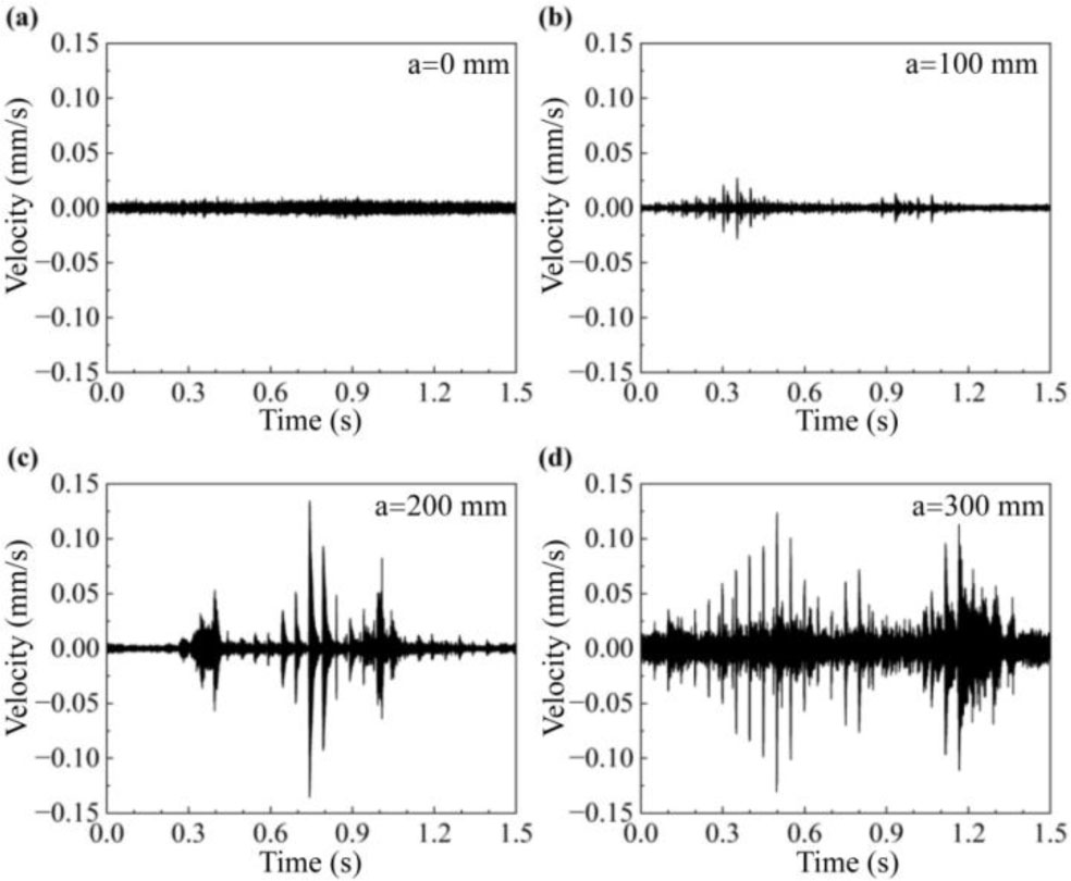
Figure 13:
Time-domain signals for different cavity sizes
Figure 14 illustrates the frequency spectra of concrete specimens with varying cavity dimensions obtained via Fast Fourier Transform (FFT). The spectrum of the solid specimen remains baseline-stable, characterized by low amplitudes and the absence of significant resonance peaks, signifying structural integrity. As the cavity diameter increases, the spectral characteristics undergo a marked transformation. Specifically, the velocity spectra acquired by the Laser Doppler Vibrometer reveal that the 100-mm cavity exhibits peaks at 2502 Hz and 4788 Hz (with amplitudes of 0.25×10⁻³ mm/s and 0.2×10⁻³ mm/s, respectively); the 200-mm cavity displays a dominant resonance at 1871 Hz (2.41×10⁻³ mm/s); and the 300-mm cavity yields peaks at 821 Hz and 4810 Hz (2.55×10⁻³ mm/s and 1.54×10⁻³ mm/s, respectively). The experimental data reveal two distinct evolutionary patterns:
(1) The characteristic frequency is inversely related to the cavity size. The dominant frequency of the 300 mm cavity is reduced by approximately 67% compared to that of the 100 mm cavity.
(2) The vibration amplitude is positively correlated with the cavity size. The amplitude of the 300 mm cavity is approximately 10 times greater than that of the 100 mm cavity.
These characteristics provide reliable quantitative indicators for the non-destructive detection of concrete defects. According to the theoretical formula for thickness vibration (Equation 7), the calculated thickness resonance frequency of the concrete specimens is approximately 5900 Hz. The deviations from the measured values – 4788 Hz (Figure 14(a)) and 4810 Hz (Figure 14(d)) – are 18.8% and 18.5%, respectively. The absence of a distinct thickness frequency peak in Figure 14(c) may be attributed to multiple reflections caused by internal aggregates, sand particles, and air voids.
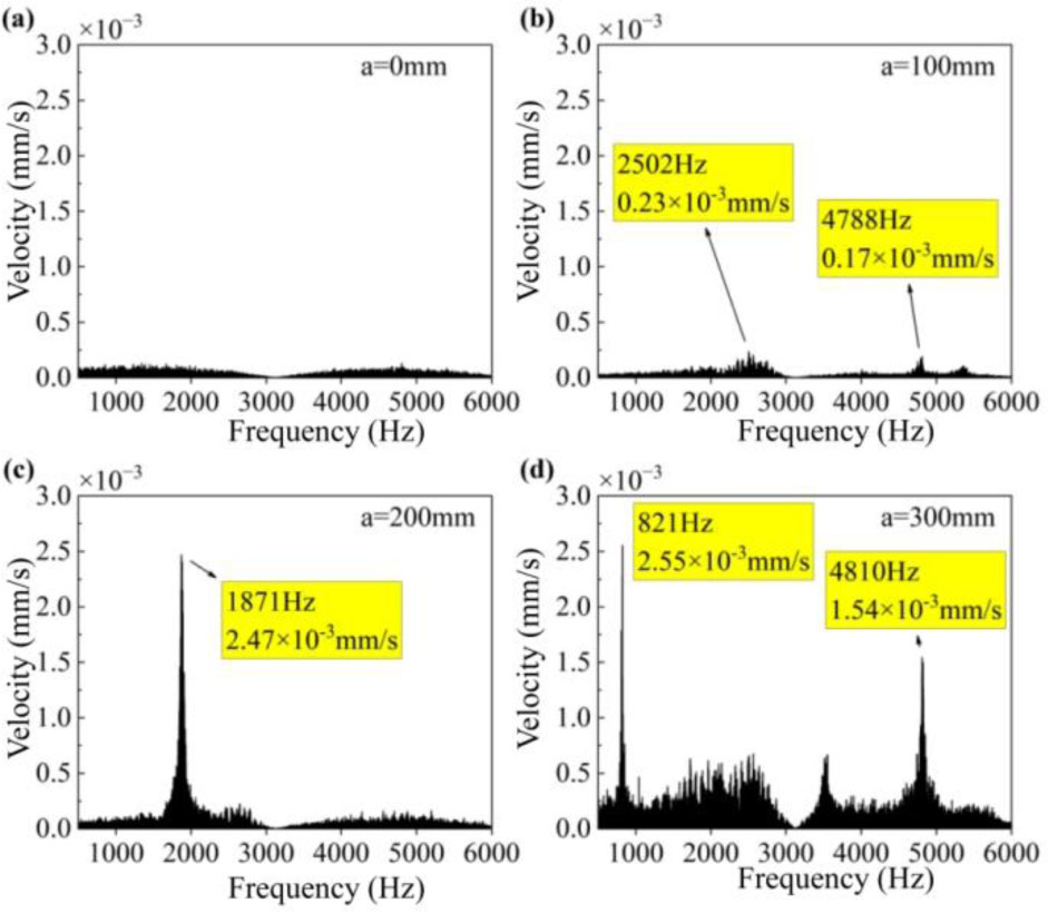
Figure 14:
Frequency spectra for different cavity sizes
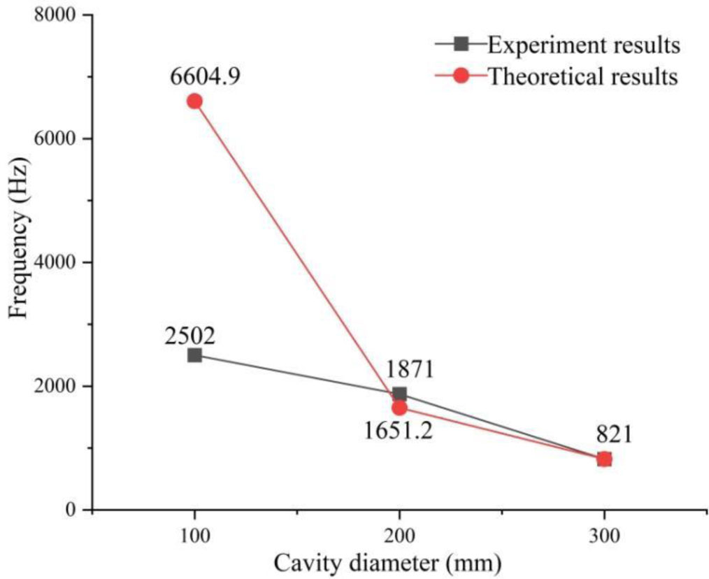
Figure 15:
Comparison of theoretical and experimental results on the effect of cavity diameter on frequency
Figure 15 compares the surface bending resonance frequencies obtained from theoretical analytical models and experimental measurements. Overall, the resonance frequency decreases progressively as the cavity diameter expands. The trends across both datasets – theoretical and those captured by the Laser Doppler Vibrometer - are highly consistent, exhibiting a pronounced negative correlation. This trend demonstrates that the cavity diameter exerts a significant influence on the vibrational signatures of the overlying concrete layer. This phenomenon is attributed to the fact that, at a constant burial depth, a larger width-to-depth ratio reduces the effective flexural stiffness of the concrete plate overlying the cavity, thereby lowering the fundamental bending resonance frequency.
5.2. Vibration Characteristics of Concrete with Different Cavity Depths
Figure 16 illustrates the time-domain surface velocity responses of concrete specimens with varying cavity depths h. Figure 16(a)–(d) display the waveforms for the solid specimen and the cavity centers at depths of 20, 50, and 80 mm, respectively. Measurements acquired by the Laser Doppler Vibrometer reveal that the solid specimen exhibits a minimal vibration amplitude (≈0.05 mm/s) and a stable waveform, signifying structural integrity. At a cavity depth of 20 mm, the vibration amplitude increases significantly, reaching a peak of 0.15 mm/s and exhibiting a pronounced fluctuation at 0.5 s. At a depth of 50 mm, the amplitude decreases slightly (to≈0.12 mm/s), with the peak fluctuation shifting earlier to 0.45 s. When the depth increases to 80 mm, the amplitude further attenuates to approximately 0.08 mm/s, accompanied by a notably smoother signal profile. These results demonstrate a clear correlation between cavity depth and vibrational response, specifically manifested as follows:
(1) The vibration amplitude decreases with increasing cavity depth – a reduction of approximately 47% from 20 mm to 80 mm.
(2) The degree of signal fluctuation weakens as the cavity depth increases.
(3) The time at which the peak occurs shifts earlier with increasing depth.
These observations suggest that deeper cavities tend to attenuate the bending resonance effect on the concrete surface, providing an important basis for evaluating the depth of internal defects in concrete structures.
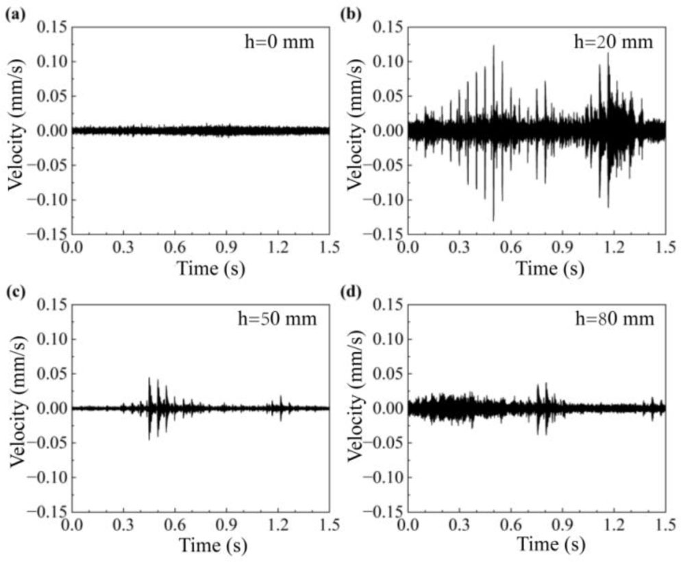
Figure 16:
Time-domain signals for different cavity depths
Figure 17 illustrates the frequency spectra of concrete specimens with varying cavity depths h. The frequency spectrum of the solid specimen remains stable, with low amplitude and no prominent peaks. As the cavity depth increases, the characteristic frequencies shift upward while the amplitudes decrease. At a depth of 20 mm, two distinct peaks appear at 821 Hz (2.55×10⁻³ mm/s) and 4810 Hz (1.54×10⁻³ mm/s); at 50 mm depth, the main peak shifts to 1989 Hz (0.8×10⁻³ mm/s), and the amplitude at 4803 Hz drops to 0.2×10⁻³ mm/s; at 80 mm depth, the frequencies further rise to 2303 Hz (0.6×10⁻³ mm/s) and 4792 Hz (0.26×10⁻³ mm/s).
The experimental data indicate that for every 30 mm increase in cavity depth, the characteristic frequency increases by approximately 500 Hz on average, while the vibration amplitude decreases by about 50%, revealing an inverse relationship between depth and frequency spectrum characteristics.
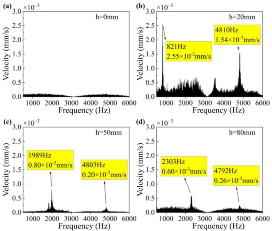
Figure 17:
Frequency spectra for different cavity depths
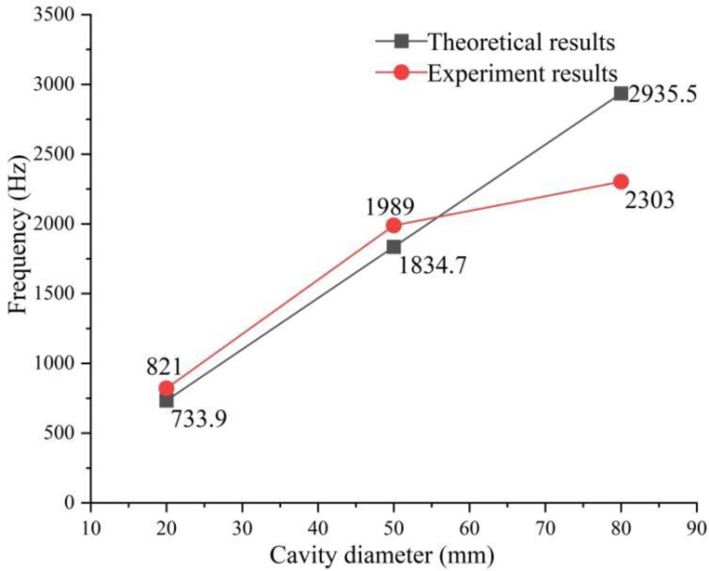
Figure 18:
Comparison of theoretical and experimental results on the effect of cavity depth on frequency
Figure 18 compares the surface bending resonance frequencies of the concrete specimens at various cavity depths, derived from both theoretical analytical models and experimental measurements. Overall, the resonance frequency increases progressively with increasing cavity depth. The trends observed in both theoretical predictions and the data captured by the Laser Doppler Vibrometer are highly consistent, exhibiting a pronounced positive correlation. This trend demonstrates that the cavity depth exerts a significant influence on the vibrational signatures of the concrete surface. For a constant cavity diameter, a decrease in the width-to-depth ratio enhances the effective flexural stiffness of the overlying concrete layer, thereby shifting the fundamental bending resonance to a higher frequency.
5.3. Vibration Characteristics of Concrete at Different Detection Distances
To evaluate the influence of stand-off distance on signal characteristics, the acoustic excitation system and the Laser Doppler Vibrometer were repositioned at a distance of 10 m from the specimens. Figure 19 presents the vibration frequency spectra of Specimens 2, 4, and 5 acquired at different stand-off distances (5 m and 10 m). For Specimen 2, the resonance frequency remained nearly stable, recorded at 1871 Hz (2.47×10⁻³ mm/s) at a 5-m stand-off distance and 1874 Hz at 10 m. while the velocity amplitude captured by the Laser Doppler Vibrometer dropped to 1.92×10⁻³ mm/s, representing a 22.3% reduction. Regarding Specimen 4, the LDV identified resonance frequencies of 1989 Hz (0.80×10⁻³ mm/s) at 5 m and 1984 Hz at 10 m. The corresponding amplitude decreased to 0.48×10⁻³ mm/s, marking a 40.0% decline. For Specimen 5, the resonance frequency exhibited a negligible shift from 2303 Hz at 5 m to 2301 Hz at 10 m. However, the amplitude diminished drastically to 0.08×10⁻³ mm/s at the 10-m distance, a significant 86.7% attenuation. All specimens exhibited the following characteristics as detection distance increased:
(1) The change in resonance frequency was minimal—less than 0.2% (maximum deviation of 3 Hz).
(2) The vibration amplitude decreased significantly with increasing distance, with the highest attenuation observed in high-frequency signals, which showed an 86.7% reduction. These results indicate that detection distance primarily affects signal strength, while having negligible impact on resonance frequency characteristics.
Detection distance has a notable influence on the vibration signals of concrete. As the distance increases, signal amplitude generally decreases, whereas resonance frequency remains relatively stable. The minimal variation in resonance frequencies across specimens suggests that the influence of cavities may be concentrated within specific vibration modes and frequency ranges. However, in long-distance measurements, the significant attenuation of signal amplitude may reduce measurement accuracy, particularly for responses with inherently low amplitude.
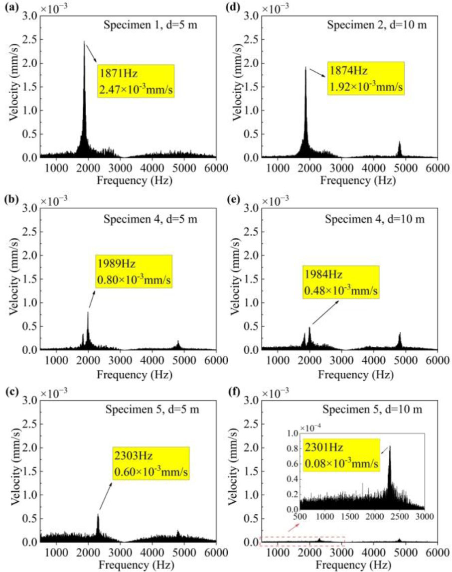
Figure 19:
Comparison of frequency spectra at different detection distances
6. Cavity Range Identification in Concrete Based on Vibration Velocity
To evaluate the capability of the Laser Doppler Vibrometer in identifying subsurface cavities a scanning grid comprising 143 measurement points (13×11) was uniformly established on the surface of Specimen 3 with a spatial resolution of 50 mm, as illustrated in Figure 20. This dense measurement layout enables the LDV to effectively capture the spatial distribution of surface velocity under acoustic excitation.
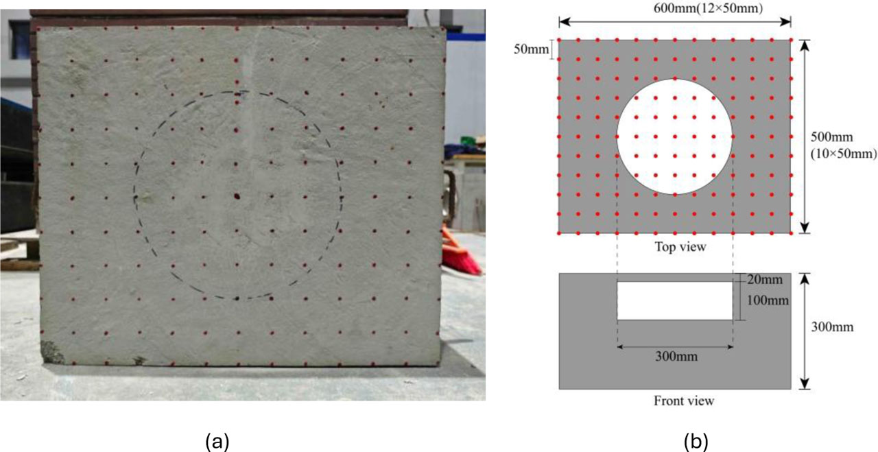
Figure 20:
Measurement point layout of the concrete specimen: (a) Photograph of the concrete specimen; (b) Layout of measurement points
Figure 21 illustrates the distribution characteristics of surface vibration velocity on the concrete specimen. The results show that the vibration velocity in the cavity region (indicated by the white dashed line) is significantly higher than in the surrounding areas, exhibiting a distinct resonance behaviour. The vibration velocity reaches its maximum at the centre of the cavity and gradually decreases outward, forming a gradient pattern. The highest velocity occurs in the central region of the specimen, indicating that the presence of the cavity reduces local stiffness and induces a pronounced amplification of vibration response.
The 3D visualization analysis clearly reveals a strong spatial correlation between the region of enhanced vibration and the actual cavity location, with a spatial match exceeding 90%. This study confirms the effectiveness of the non-destructive detection method based on acoustic excitation and LDV technology. The spatial distribution of the vibration velocity field can serve as a key indicator for diagnosing internal defects in concrete, offering a new technical approach for structural health monitoring in engineering applications.
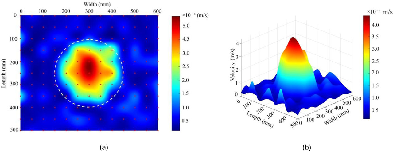
Figure 21:
Distribution characteristics of surface vibration velocity on the concrete specimen. (a) 2D Distribution (b) 3D distribution
7. Potential Limitations and Future Work
While the integration of acoustic excitation and LDV demonstrates high precision for cavity detection, several practical limitations should be noted.
(1) Environmental noise in operational tunnels – such as vehicle-induced vibrations and aerodynamic noise – presents a challenge for capturing subtle structural responses.
(2) As experimental results show, the vibration amplitude attenuates significantly as the detection distance increases to10m, potentially reducing the detection accuracy for low-amplitude features in far-field scenarios.
(3) The optical nature of LDV requires a relatively clear line-of-sight and stable surface reflection; therefore, the presence of heavy dust or water films on the lining surface may necessitate pre-cleaning or signal compensation. Future work will focus on developing adaptive noise-reduction algorithms and investigating the impact of reinforcement density on multi-modal resonance behaviour.
8. Conclusion
(1) The integrated approach using acoustic excitation and the Laser Doppler Vibrometer demonstrates superior performance in tunnel lining inspections. Compared to hammer impact, it yields more stable responses across a broader frequency spectrum while eliminating contact-induced damage.
(2) An increase in cavity size leads to a decrease in bending resonance frequency and an increase in vibration amplitude, while greater cavity depth results in higher frequencies and reduced amplitudes. When the diameter-to-depth ratio exceeds a certain threshold, longitudinal waves are fully reflected at the cavity boundary, generating a distinct low-frequency bending resonance peak. This pattern provides a theoretical basis for the quantitative assessment of defects.
(3) A comparison of experimental data at different detection distances shows that increased distance causes attenuation of vibration amplitude, while the shift in resonance frequency remains minimal. This characteristic suggests that while signal gain must be optimized for remote measurements, frequency features remain reliable indicators for defect identification.
(4) LDV coupled with acoustic excitation can precisely capture micro-vibrations on concrete surfaces. The 3D spatial distribution of vibration velocity corresponding to resonance frequencies clearly outlines the cavity boundaries. The vibration amplitude shows a gradient decay from the cavity centre outward, eventually returning to background levels – validating the method's capability in spatial defect identification.
Acknowledgments
The authors would like to acknowledge the support of the Key Project for Technological Innovation and Application Development in Chongqing (CSTB2025TIAD-KPX0029), the National Natural Science Foundation of China (No.52274176), the Guangdong Province Key Areas R & D Program (2022B0101070001), Chongqing Elite Innovation and Entrepreneurship Leading talent Project (CQYC20220302517), the Chongqing Municipal Education Commission "Shuangcheng Economic Circle Construction in Chengdu-Chongqing Area" Science and Technology Innovation Project (KJCX2020031), the Research Project of Chongqing Water Resources Bureau (CQSLK-2025005), the Natural Science Foundation of Chongqing (CSTB2024NSCQ-MSX0744).
Notes
[1] Contributed by Author Contributions
[L.L.] conceived and designed the study. [H.L.R.] conducted the experiments and collected the data. [Y.W.] performed the statistical analysis. [L.M.] contributed to data interpretation and manuscript drafting. [F.T.] performed the statistical analysis. [J.D.] contributed to data interpretation and manuscript drafting. [Z.H.Z.] contributed to data interpretation and manuscript drafting. [H.Y.Y.] contributed to data interpretation and manuscript drafting, performed the statistical analysis. [Y.C.G.] designed the study and supervised the project.
All authors critically reviewed and approved the final version of the manuscript and agreed to be accountable for all aspects of the work.