

1. Introduction
Mixing quality in drinking water and wastewater treatment plants (DWTPs and WWTPs) directly affects the effectiveness and economic performance of processes that rely on it (Aanjaneya & Agrawal, 2023; Shira, 2022). This is especially true for coagulation and flocculation (C&F) – processes that are both highly sensitive to local hydrodynamics and critically important for overall treatment performance (Bratby, 2016; Pivokonský et al., 2019). The design and assessment of C&F mixing has historically relied on the global averaged velocity gradient Ḡ, introduced by Camp and Stein (Camp & Stein, 1943), which lumps the spatially heterogeneous hydrodynamic environment into a single number derived from the volume-averaged rate of turbulent kinetic energy dissipation ɛ̅:
Where:ν - the kinematic viscosity.
This parameter was introduced to substitute the local absolute velocity gradient GA – at the time incomputable – that captures the actual hydrodynamic environment experienced by individual flocs:
Where:u, v and w – the velocity components in the x, y, and z directions, respectively, and the cross-derivative terms represent the shear rates acting on a fluid element.
Although Ḡ was widely adopted in practice, it was never mathematically justified as a substitute for GA (Kramer & Clark, 1997) and was criticized for obscuring the local-scale processes that govern floc fate (Clark, 1985; Cleasby, 1984; Pedocchi & Piedra-Cueva, 2005). The physical reason is rooted in the turbulent energy cascade: turbulent kinetic energy (TKE) generated at the scale of the impeller is transferred through the inertial subrange down to the Kolmogorov microscale, where it is dissipated as heat. This dissipation is physically realized through local velocity gradients – the spatial derivatives of the velocity field – which impose shear and extensional stresses on suspended flocs. The size and structural integrity of a floc are therefore governed by the local dissipation rate ɛ: flocs smaller than the Kolmogorov microscale experience viscous shear on their surface, while those comparable to or larger than the dissipative eddies are subject to pressure-driven fragmentation (Lu et al., 1998; Soos et al., 2008). Crucially, whether a floc survives or breaks depends not only on the local gradient it encounters but also on the hydrodynamic conditions under which it was formed – a floc aggregated under gentle mixing possesses lower cohesive strength and will fragment at gradients that a floc formed under more intense conditions would withstand (Bubakova et al., 2013; Spicer & Pratsinis, 1996). Experimental studies place the transition from aggregation-dominated to break-up-dominated regimes around GA = 80–200 s−1 (Bouyer et al., 2004; Bubakova et al., 2013), and two vessels sharing identical Ḡ can produce fundamentally different flocculation outcomes if their spatial distributions of local gradients differ.
The most instructive demonstration comes from Balemans et al. (Balemans et al., 2020), who compared jar tests using radial and axial impellers supplemented with CFD modelling. At 70 rpm, the radial impeller produced Ḡ = 50 s−1 with Gmax = 257 s−1, while the axial impeller yielded Ḡ = 17 s−1 with Gmax = 180 s−1. Based on either parameter alone, one would expect the radial impeller to produce more vigorous flocculation; the opposite was observed. The explanation lies in the cumulative distribution of local velocity gradients: the radial impeller exposes a large volume fraction to destructive shear, while the axial impeller confines its highest gradients to a negligible region near the blades. This finding could not be explained by Ḡ, Gmax, or the 95th-percentile gradient – all single-number surrogates that discard the spatial information essential to understanding floc fate.
1.1. Recent Advances in CFD Modelling of Stirred-Tank Hydrodynamics
The choice of turbulence closure for stirred-tank CFD remains actively debated, particularly when the quantities of interest extend beyond bulk mixing metrics to spatially resolved velocity gradients. The standard k–ɛ model has long served as the default in water-treatment CFD owing to decades of calibration for Rushton turbine geometries (Joshi et al., 2011), but recent comparative studies have exposed its limitations for derivative quantities. A recent study (Ben Kilani et al., 2025) confirmed that k–ɛ reproduces mean velocity profiles with high accuracy at moderate Reynolds numbers, yet showed that turbulent kinetic energy – and by extension the local dissipation rate from which velocity gradients are inferred – Is systematically underpredicted in the impeller discharge zone. (Chatila & Danageuzian, 2022) compared the k–ω SST and IDDES (Improved Delayed Detached Eddy Simulation) closures against PIV measurements in a paddle flocculator and found that while IDDES offered only marginal improvement in bulk velocity prediction, it captured secondary flow structures that SST smoothed out – structures directly responsible for local shear peaks.
Scale-resolving approaches have matured rapidly. For example, a study validated a Lattice-Boltzmann LES (LB-LES) implementation against 4D particle tracking velocimetry in a stirred bioreactor and demonstrated that LB-LES reproduces trailing vortex structures and mixing-time distributions with less than 11% deviation from experiment – performance comparable to or better than RANS at a fraction of the setup effort (Kuschel et al., 2021). Another study extended LBM validation to multiple impeller types (Rushton and pitched-blade turbines) across laminar-to-turbulent regimes, confirming that GPU-accelerated LBM predicts power numbers, local velocity components, and dissipation-rate distributions in good agreement with published experimental data (Kersebaum et al., 2024). It has been also demonstrated that such GPU-accelerated LBM-LES implementations make industrially relevant lattice resolutions feasible within hours, removing the traditional computational-cost barrier that limited LES adoption in engineering practice (Miller et al., 2025).
Despite these advances, systematic head-to-head comparisons between multiple RANS closures and LBM-LES for the same geometry remain scarce. Hartmann et al. compared LES and RANS against laser-Doppler anemometry in a Rushton tank but did not examine velocity gradients (Hartmann et al., 2004). Gotfredsen et al. validated RANS and DES for pipe-flow mixing without extending the analysis to local shear rates (Gotfredsen et al., 2020). Weiland et al. studied Lagrangian transport and mixing in a stirred tank but focused on residence-time statistics rather than the gradient field (Weiland et al., 2023). None of these studies quantified how turbulence-model errors propagate from velocities into the derived gradients that govern flocculation.
1.2. Local Velocity Gradients, Floc Fate, and the Limitations of Ḡ
The inadequacy of the global mean velocity gradient Ḡ as a flocculation design parameter has been demonstrated from multiple angles. Balemans et al. showed that two impeller configurations sharing the same Ḡ produce fundamentally different cumulative distributions of local G – and correspondingly different floc properties in high-rate activated sludge reactors (Balemans et al., 2020). Zhan et al. coupled CFD with a population balance model (PBM) for a mechanical flocculator and found that floc size predictions depend critically on the spatial resolution of the local velocity gradient field: replacing the spatially resolved G with its volume average changed the predicted median floc diameter by up to 40% (Zhan et al., 2021).
Experimental breakage studies reinforce this picture. Soos et al. and Bubakova et al. identified a shear-rate threshold of approximately 80–200 s−1 separating aggregation-dominated from breakage-dominated regimes in stirred tanks (Bubakova et al., 2013; Soos et al., 2008). Bubakova et al. in particular further demonstrated that floc cohesive strength depends on the hydrodynamic history of formation, meaning that the spatial distribution of gradients – not just the peak or the mean – determines long-term floc fate (Bubakova et al., 2013)
Most recently, Bridgeman and Dapelo argued that even the local velocity gradient G may not be the optimal design parameter: their CFD-based analysis of hydraulic flocculators found that volume-weighted vorticity correlates more strongly with both floc size and floc strength than the Camp number or Ḡ (Bridgeman & Dapelo, 2025). While their proposal targets a different class of flocculator (hydraulic rather than mechanical), it underscores a broader point: the conventional single-parameter framework is being challenged from multiple directions, and any CFD-informed alternative – whether based on G distributions, vorticity, or dissipation rate – requires a turbulence model whose local predictions can be trusted. Quantifying that trust across different closure strategies is the central objective of the present work.
1.3. Validation Benchmarks and the Present Contribution
Rigorous multi-model validation requires high-quality experimental data with quantified uncertainties. Sommer et al. assembled a particularly comprehensive dataset for this purpose: stereoscopic PIV measurements in a standard baffled Rushton turbine tank at multiple Reynolds numbers, with full statistical uncertainty quantification and an openly available database (Sommer et al., 2021). Chatila and Danageuzian similarly provided PIV-validated CFD data for a paddle flocculator, though limited to two turbulence models (Chatila & Danageuzian, 2022). The availability of such open datasets creates an opportunity – not yet exploited – for systematic multi-model validation that extends beyond velocity profiles to derived quantities.
The present study addresses this opportunity. Four turbulence modelling approaches – standard k–ɛ, k–ω SST, and RSM (finite-volume RANS in Siemens STAR-CCM+), alongside LBM-LES (M-Star CFD) – are validated against the Sommer et al. PIV benchmark (Sommer et al., 2021). Critically, the comparison proceeds from velocity profiles through derived velocity gradients to floc-breakage threshold exceedance, quantifying the systematic amplification of model errors at each stage. To the authors' knowledge, this is the first study to compare RANS and LBM-LES paradigms at the level of local velocity gradients in a flocculation-relevant geometry, providing practitioners with evidence-based guidance for turbulence model selection in CFD-informed flocculator design.
The present study examines how large this difference is in practice. Four turbulence modelling approaches – three finite-volume RANS closures (standard k–ɛ, k–ω SST, and Reynolds Stress Model or RSM) implemented in Siemens STAR-CCM+, and one LBM-LES solver (M-Star CFD) – are validated against a publicly available PIV dataset for a Rushton turbine stirred tank (Sommer et al., 2021). Beyond comparing mean velocity profiles, the analysis focuses specifically on how velocity prediction errors propagate into the local velocity gradients that govern floc fate, and whether the spatial distribution of the predicted velocity field captures the heterogeneity that single-number metrics cannot.
2. Methodology
2.1. Research Design
The study follows a validation-first comparative design: CFD simulations of two distinct turbulence-modelling paradigms – finite-volume RANS and lattice-Boltzmann LES – are evaluated against a publicly available, experimentally measured velocity field for a mechanically stirred tank. The experimental dataset was selected on the criterion that it satisfies the requirements of “CFD-grade” data as defined by (Sommer et al., 2021): spatially resolved mean and fluctuating velocity fields with quantified measurement uncertainties, covering a range of operating conditions, and made openly accessible for model validation purposes. The comparison is restricted to the single-phase, time-averaged liquid velocity field, which constitutes the hydrodynamic basis relevant to C&F applications and admits the most direct and unambiguous comparison between simulation and measurement.
2.2. Materials and Procedures
2.2.1. Validation Benchmark
Even recent CFD and experimental work published in this journal alone – spanning vertical-drop hydraulics (Shaikhli et al., 2024) and spatially varied open-channel flows (Hasan & Almajeed A Alabas, 2026) – has underscored the continued importance of rigorous experimental validation of turbulence closures, a principle that guides the RANS-vs-LBM-LES comparison presented here.
The experimental reference dataset is drawn from (Sommer et al., 2021), who assembled a CFD-grade database for solid–liquid flow in a cylindrical baffled stirred tank of diameter Dt = 90 mm, stirred by a Rushton turbine of diameter Di = Dt/3 = 30 mm. The impeller clearance from the tank bottom is Ci = Dt/3, and four baffles of width W_baf = Dt/10 are equally spaced along the tank wall. The liquid height is H = Dt, giving a filled volume characteristic of standard stirred-tank configurations. Full geometric details, including blade and disk dimensions, are given in Fig. 1 of the mentioned study (Sommer et al., 2021).
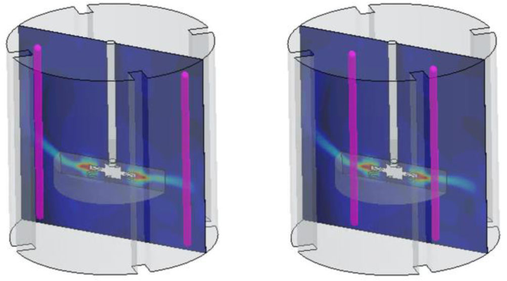
Figure 1:
Line-probes (in purple) used to extract the axial profiles of the radial velocity components in STAR CCM+
Two single-phase operating conditions are used as validation targets: impeller rotation speed Ω = 650 rpm (with Reynolds number based on particle rotation rate ReΩ = ΩDi2/ν = 9717) and Ω = 1500 rpm (ReΩ = 22 424), where the latter approaches the threshold for fully developed turbulent flow conventionally placed at ReΩ ≈ 20 000 (Bittorf & Kresta, 2000). Liquid velocities are reported normalized by the impeller tip velocity utip = πΩDi.
Velocity fields were measured using Particle Image Velocimetry (PIV) with fluorescent PMMA tracers (particle diameter dp = 20–50 μm, St ≪ 0.1) illuminated by a Nd:YLF laser sheet of 1 mm thickness, captured at 4500 frames/s with a spatial resolution of 0.06 mm/pixel. The measurement plane is located at azimuthal angle θ = 0°, midway between two baffles, and covers half the tank radius, taking advantage of flow symmetry. Instantaneous velocity fields were time-averaged over 50 impeller rotations, yielding between 9 000 and 21 000 time steps per condition; statistical uncertainty was quantified per Equation (13) of (Sommer et al., 2021) and is reported alongside all velocity data in the open database (Sommer et al., 2021). The present study uses the time-averaged radial velocity profiles at two radial positions, 2r/Dt = 0.44 (near-impeller discharge) and 2r/Dt = 0.80 (near-wall region), at both operating conditions.
PIV Database Correction
During the preparation of the present study, a systematic discrepancy was identified between the radial coordinate column of the publicly released PIV database and the velocity profiles published in the accompanying paper (Sommer et al., 2021). The database column labelled twoR_per_Dt – ostensibly representing the dimensionless radial coordinate 2r/Dt - spans from − 0.028 to 0.507 across 100 unique radial positions. Two independent lines of evidence demonstrate that this column in fact contains r/Dt values rather than 2r/Dt. First, the position 2r/Dt = 0.80, at which Sommer et al. explicitly present velocity profiles (their Figs. 10 and 14), does not exist in the database if the column is taken at face value, since the maximum stored value is 0.507; interpreting the column as r/Dt yields a maximum true 2r/Dt of 1.014, i.e. coverage from the tank centre to the wall, which is consistent with both the stated scope of the database and the full-radius contour plots presented in Fig. 8 of the same paper. Second, quantitative comparison of the extracted peak radial velocities confirms the factor-of-two offset: the profile at database coordinate 0.22 yields a peak ūr/utip = 0.397 at Ω = 650 rpm, matching the value of approximately 0.40 readable from Figure 9 at the position labelled 2r/Dt = 0.44, whereas the profile at database coordinate 0.44 gives a peak of only 0.170 - less than half of the published value. An analogous match holds at the second extraction position: database coordinate 0.40 reproduces the published profile at 2r/Dt = 0.80 (peak ūr/utip ≈ 0.24), while coordinate 0.80 is altogether absent from the database. The correspondence 0.22 × 2 = 0.44 and 0.40 × 2 = 0.80 is exact. Accordingly, all radial coordinates extracted from the open database in this work have been multiplied by a factor of two to recover the true dimensionless position 2r/Dt consistent with the notation used throughout (Sommer et al., 2021).
2.2.2. RANS Model (Siemens Star CCM+)
RANS simulations were performed in Siemens STAR-CCM+ (version 2510.0001, build 20.06.010). The computational domain reproduces the geometry of (Sommer et al., 2021) described above. The fluid domain was discretized using a polyhedral mesh of approximately 611 000 cells, with prism layer refinement at all solid walls to resolve the near-wall velocity gradient. A grid independence study was performed to confirm that the reported results are mesh-converged.
Impeller rotation was handled using the Moving Reference Frame (MRF) approach with a mixing-plane interface, following the same configuration adopted by Sommer et al. in their cross-validation simulations. This method couples a rotating inner zone enclosing the impeller to a stationary outer zone comprising the remainder of the fluid domain, with circumferentially averaged quantities passed across the interface.
Three turbulence closures were assessed: (a) the standard k–ɛ model with standard wall functions, representing the most widely used two-equation closure in water-sector CFD practice; (b) the k–ω SST (Shear Stress Transport) model of Menter (1994), which blends k–ω behaviour in the near-wall region with k–ɛ behaviour in the outer flow and includes a stress limiter to improve performance in adverse pressure gradients and separated flows; and (c) the Reynolds Stress Model (RSM), which solves individual transport equations for all six independent Reynolds stress components rather than relying on the Boussinesq eddy-viscosity hypothesis, thereby capturing stress anisotropy and rotational effects more faithfully. The inclusion of RSM is consistent with the turbulence model employed by (Sommer et al., 2021) in their own single-phase validation, which facilitates direct comparison. No-slip boundary conditions were applied at all solid walls; a free-slip condition was imposed at the top liquid surface, treated as flat. Simulations were run to steady state; convergence was assessed by monitoring residuals of all transport equations and the global mass imbalance, with the solution accepted once all residuals fell below 10−4 and showed no further systematic trend.
Post-processing extracted axial profiles of the time-averaged radial velocity component, ūr/utip, at 2r/Dt = 0.44 and 2r/Dt = 0.80, corresponding to the experimental sampling locations (Figure 1). The data were extracted from both probes and subsequently combined in an averaged series. In the stationary MRF zone, time-averaged quantities are obtained directly; in the rotating zone, circumferential averaging over all blade angles was applied to obtain values comparable to the time-averaged experimental data, following the procedure described in (Sommer et al., 2021).
All three closures solve the steady, incompressible RANS equations on the same 611 k polyhedral mesh. The standard k–ɛ model (Launder & Spalding, 1974) and k–ω SST (Menter, 1994) are both Boussinesq eddy-viscosity closures, while the Reynolds Stress Model transports each component of the Reynolds-stress tensor directly with the linear pressure–strain closure of Gibson & Launder – avoiding the isotropic-viscosity assumption that is questionable in the anisotropic impeller jet.
Near walls, log-law wall functions are applied; the area-averaged y+ on the impeller blades stayed in the range 35–95 across all speeds. Convergence required scaled residuals below 10−4 together with impeller torque stable to within ±0.5 % over 2000 successive iterations (depending on the RPM).
2.2.3. Lattice-Boltzmann LES Simulation (M-Star CFD)
LBM-LES simulations were performed in M-Star CFD. The computational domain is a cubic lattice spanning (−0.045, 0, −0.045) m to (0.045, 0.09, 0.045) m in the x, y, and z directions, respectively, reproducing the 90 mm tank geometry of Sommer et al. (2021). The domain is set to PartialFill mode with a fill height of 0.09 m (= H = Dt), consistent with the experimental liquid height. Gravity is applied in the negative y-direction at 9.81 m·s−2.
The lattice resolution is 240 × 240 × 240 nodes, yielding a uniform lattice spacing of dx = 3.75 × 10⁻⁴ m and a total of 13.8 × 10⁶ lattice sites. The D3Q19 velocity set is used. The time step is determined by co-specifying the Courant number at 0.1, giving dt = 3.66 × 10⁻⁵ s. The impeller is represented using the Immersed Boundary (IB) method, with a reference diameter of 0.03007 m ≈ Di, and a rotation axis aligned with the y-direction. Simulations were run for two impeller speeds: Ω = 650 rpm and Ω = 1500 rpm, matching the experimental conditions of (Sommer et al., 2021).
Turbulence is modelled using LES with the Smagorinsky subgrid-scale model, with a Smagorinsky coefficient of Cs = 0.1. The fluid is treated as Newtonian with density ρ = 1000 kg·m−3 and kinematic viscosity ν = 1 × 10⁻⁶ m2·s−1 (water at 25°C), consistent with the experimental working fluid.
Boundary conditions mirror those applied in the RANS simulations: no-slip conditions are imposed on all solid surfaces (tank walls, baffles, and impeller geometry) and a free-slip condition is applied at the top face of the domain, representing the flat liquid surface. Total simulation time is 20 s; time-averaging of the velocity field commences at t = 10 s, once the flow has reached a statistically stationary state, and continues uniformly over the remaining 10 s using a sampling interval of every time step. Post-processing extracted time-averaged radial velocity profiles at the same radial positions used for the RANS comparison: 2r/Dt = 0.44 and 2r/Dt = 0.80.
The M-Star solver advances particle distribution functions on a D3Q19 lattice through alternating streaming and BGK collision steps:
Where:fi - the particle distribution function associated with the i-th discrete lattice velocity ei,
δt - the lattice time step,
Ωi - the BGK single-relaxation-time collision operator.
The incompressible Navier–Stokes equations are recovered at the macroscopic scale through a Chapman–Enskog expansion (Chen & Doolen, 1998). The peak lattice Mach number is utip/cs≈0.024, comfortably within the weakly-compressible regime, and the impeller diameter is resolved by 80 lattice cells — above the Di/δx>75 guideline (Kuschel et al., 2021).
Subgrid stresses are closed with a constant-coefficient Smagorinsky model (Cs=0.1, filter width δx). The impeller geometry is rotated rigidly through the static lattice via a direct-forcing immersed-boundary method, giving a transient representation of the trailing vortices that the steady RANS closures cannot resolve by construction.
2.3. Comparison Methodology
All velocity components extracted from the CFD simulations and from the PIV dataset of (Sommer et al., 2021) are normalized by the impeller tip velocity utip = π·N·Di, where N is the impeller rotational speed (s−1) and Di = 30 mm is the impeller diameter, yielding utip = 1.021 m/s at 650 rpm and utip = 2.356 m/s at 1500 rpm. This normalization removes the explicit dependence on operating speed, rendering the velocity profiles dimensionless and enabling direct inter-comparison between the two Reynolds numbers investigated and across the four modelling approaches.
Velocity profiles are extracted along the vertical axis at two radial positions that match the PIV measurement lines reported by Sommer et al.: 2r/Dt = 0.44, located in the impeller discharge region midway between the shaft and the tank wall, and 2r/Dt = 0.80, located in the near-baffle region. For the RANS simulations the profiles are sampled at θ = 0° in the MRF reference plane. For the LBM-LES simulations, the time-averaged three-dimensional velocity field is sampled at the same radial positions in the PIV measurement plane. The axial coordinate is presented as z/H, spanning the full liquid height from the tank floor (z/H = 0) to the free surface (z/H = 1).
Because the CFD models and the PIV database use different spatial discretizations, a common comparison grid is required. The PIV experimental z/H grid (approximately 160 points) serves as the reference, and each CFD velocity profile is linearly interpolated onto this grid. Prior to interpolation, all STAR-CCM+ profiles are sorted by the axial coordinate to ensure monotonicity, as the exported data do not necessarily preserve spatial ordering. CFD values at PIV grid points that fall outside the CFD profile's axial extent are excluded from the comparison.
Agreement between each CFD model and the PIV reference data is quantified by the normalized root-mean-square deviation (NRMSD), defined for a given velocity component at extraction line k as:
Where:M - the number of valid comparison points along the profile,
u*CFD and u*PIV - the CFD-predicted and PIV-measured normalized velocities, respectively,
δu*PIV = max(u*PIV) − min(u*PIV) is the range of the PIV profile used for normalization.
This metric is computed separately for each radial position and each Reynolds number condition, yielding a set of scalar indicators that allow a structured and objective comparison of the predictive accuracy of the RANS (k–ɛ, k–ω SST, and RSM) and LBM-LES models against experiment.
2.3.1. Velocity Gradient Computation
Local velocity gradients ∂ur/∂z are computed from the interpolated radial velocity profiles using second-order central finite differences in the interior of the domain:
Where:u and z - in physical units (m/s and m, respectively), obtained by multiplying the normalized velocity by utip and the normalized axial coordinate by H = 0.090 m.
One-sided differences are used at the boundary nodes. These gradient profiles provide a direct proxy for the local shear rate experienced by fluid microstructures and flocs, which is the quantity of primary relevance to the coagulation and flocculation processes discussed in the Introduction.
A key feature of this derivative-based comparison is gradient amplification: because the gradient operator involves differences of neighbouring velocity values divided by a small spatial increment, even moderate velocity errors can produce substantially larger relative errors in the computed gradient. This effect is quantified by comparing the peak gradient from each CFD model against the corresponding PIV peak gradient, expressed as a relative error.
3. Results
3.1. Radial Velocity Profiles
Figures below (Figure 2 and 3) present the normalized radial velocity profiles ūr/utip as a function of z/H at all four combinations of impeller speed (Ω = 650 and 1500 rpm) and radial position (2r/Dt = 0.44 and 0.80), comparing the PIV reference data against the four CFD models: k–ɛ, RSM, k–ω SST, and M-Star LBM-LES.
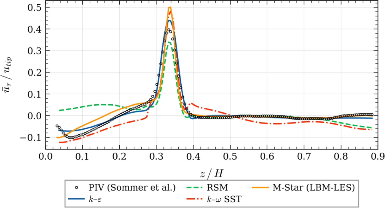
Figure 2:
Normalized radial velocity profiles at 2r/Dt = 0.44, Ω = 650 rpm
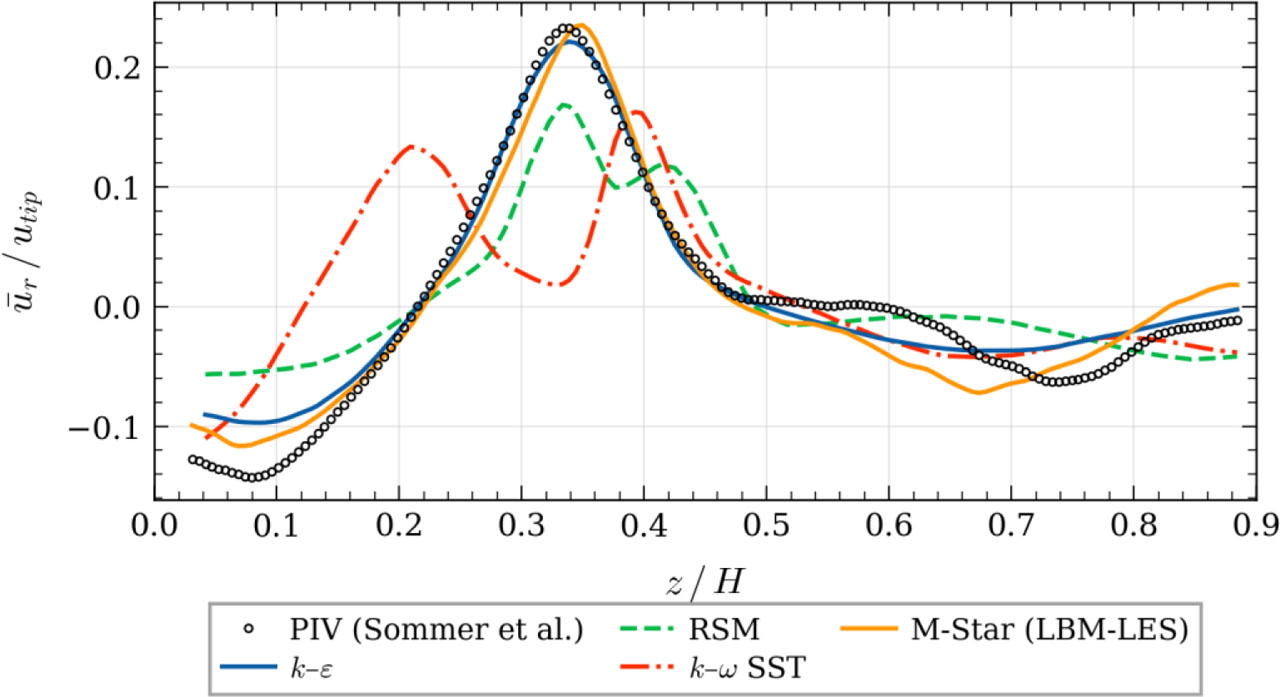
Figure 3:
Normalized radial velocity profiles at 2r/Dt = 0.80, Ω = 650 rpm
At the near-impeller position 2r/Dt = 0.44 and Ω = 650 rpm (Figure 2), all four CFD models correctly reproduce the characteristic Rushton turbine radial jet centred at z/H ≈ 0.33 (the impeller plane). The PIV reference profile exhibits a sharp peak of ūr/utip = 0.397. The k–ɛ model predicts a peak of 0.440 (+10.8% overestimation), while the RSM underpredicts the peak at 0.339 (−14.5%). Both k–ω SST (0.482, +21.5%) and M-Star (0.501, +26.3%) overestimate the peak velocity, with M-Star showing the highest peak value among all models.
At the near-wall position 2r/Dt = 0.80 (Figure 3), the radial jet has decayed considerably, with the PIV peak dropping to 0.232. Here M-Star provides the closest match (peak = 0.235, error +1.1%), followed by k–ɛ (0.221, −4.9%). Both RSM and k–ω SST underpredict the peak substantially, with errors of −27.6% and −30.1%, respectively. Notably, k–ω SST also shifts the peak location upward (z/H ≈ 0.393 vs 0.339 for PIV), indicating a misrepresentation of the jet spreading pattern.
At 1500 rpm, the near-impeller position (Figure 4) shows a qualitatively similar pattern with a PIV peak of 0.347. All four CFD models overpredict the peak velocity at this condition, with k–ɛ closest at 0.439 (+26.6%), followed by RSM (+42.1%), M-Star (+45.2%), and k–ω SST (+45.6%).
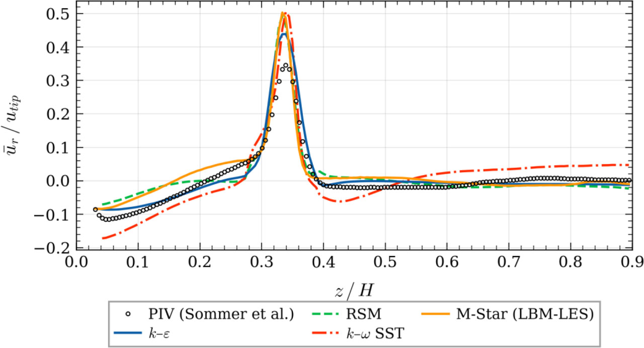
Figure 4:
Normalized radial velocity profiles at 2r/Dt = 0.44, Ω = 1500 rpm
At the near-wall position at 1500 rpm (Figure 5), the PIV peak is 0.242. M-Star again provides the closest agreement (−1.4%), while k–ɛ underpredicts moderately (−10.4%). RSM shows both the largest peak error (−18.0%) and a notable shift in peak location (z/H = 0.284 vs 0.344 for PIV).
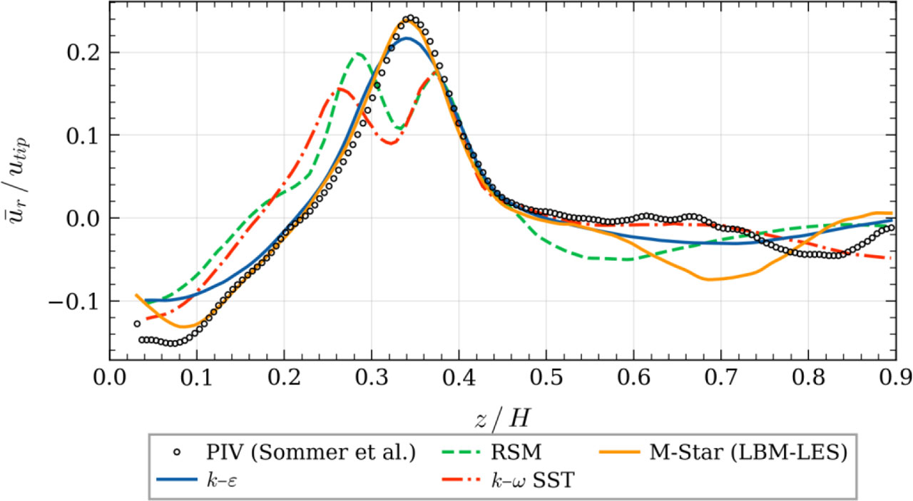
Figure 5:
Normalized radial velocity profiles at 2r/Dt = 0.80, Ω = 1500 rpm
3.2. Normalized Root-Mean-Square Deviation (NRMSD)
Table 1 summarizes the NRMSD values for the normalized radial velocity component across all eight condition–position combinations and all four turbulence models.
Table 1:
NRMSD of the normalized radial velocity ūr/utip for each CFD model, radial position, and impeller speed
| Condition | k–ɛ | RSM | k–ω SST | M-Star LBM |
|---|---|---|---|---|
| 650 rpm, 2r/Dt = 0.44 | 0.035 | 0.116 | 0.081 | 0.056 |
| 650 rpm, 2r/Dt = 0.80 | 0.051 | 0.119 | 0.213 | 0.058 |
| 1500 rpm, 2r/Dt = 0.44 | 0.065 | 0.080 | 0.094 | 0.079 |
| 1500 rpm, 2r/Dt = 0.80 | 0.057 | 0.127 | 0.112 | 0.072 |
| Average | 0.052 | 0.110 | 0.125 | 0.066 |
The k–ɛ model achieves the lowest average NRMSD across all conditions (0.052), followed by M-Star LBM-LES (0.066). RSM and k–ω SST exhibit substantially higher average NRMSD values of 0.110 and 0.125, respectively. The ranking of the four models is broadly consistent across both impeller speeds, although the relative margin between k–ɛ and M-Star narrows at 1500 rpm.
At the near-impeller position (2r/Dt = 0.44), where the radial jet is strongest and most challenging to predict, k–ɛ leads with NRMSD values of 0.035 (650 rpm) and 0.065 (1500 rpm). At the near-wall position (2r/Dt = 0.80), M-Star and k–ɛ are comparably accurate, while k–ω SST performs notably poorly at 650 rpm (NRMSD = 0.213).
3.3. Peak Velocity Errors
The peak velocity errors (Table 2) reveal important asymmetries in model behaviour. At the near-impeller position, most models tend to overpredict the peak, with k–ω SST and M-Star showing the largest overpredictions (up to +46%). RSM, by contrast, underpredicts the peak at 650 rpm (−14.5%) but overpredicts it at 1500 rpm (+42.1%), suggesting a Reynolds-number sensitivity in its closure behaviour. At the near-wall position, where the jet has diffused, underprediction is more common, with RSM and k–ω SST producing peak errors exceeding – 25% at some conditions.
Table 2:
Peak normalized radial velocity and relative error for each CFD model
| Condition | PIV peak | k–ɛ | RSM | k–ω SST | M-Star |
|---|---|---|---|---|---|
| 650 rpm, 0.44 | 0.397 | 0.440 (+10.8%*) | 0.339 (−14.5%) | 0.482 (+21.5%) | 0.501 (+26.3%) |
| 650 rpm, 0.80 | 0.232 | 0.221 (−4.9%) | 0.168 (−27.6%) | 0.162 (−30.1%) | 0.235 (+1.1%) |
| 1500 rpm, 0.44 | 0.347 | 0.439 (+26.6%) | 0.492 (+42.1%) | 0.505 (+45.6%) | 0.503 (+45.2%) |
| 1500 rpm, 0.80 | 0.242 | 0.217 (−10.4%) | 0.198 (−18.0%) | 0.175 (−27.7%) | 0.239 (−1.4%) |
3.4. Local Velocity Gradients
The local velocity gradients were computed according to the methodology expounded in Section 2.3.1 of the article. The Figure 6 and Figure 7 show their distribution over the axial profiles.
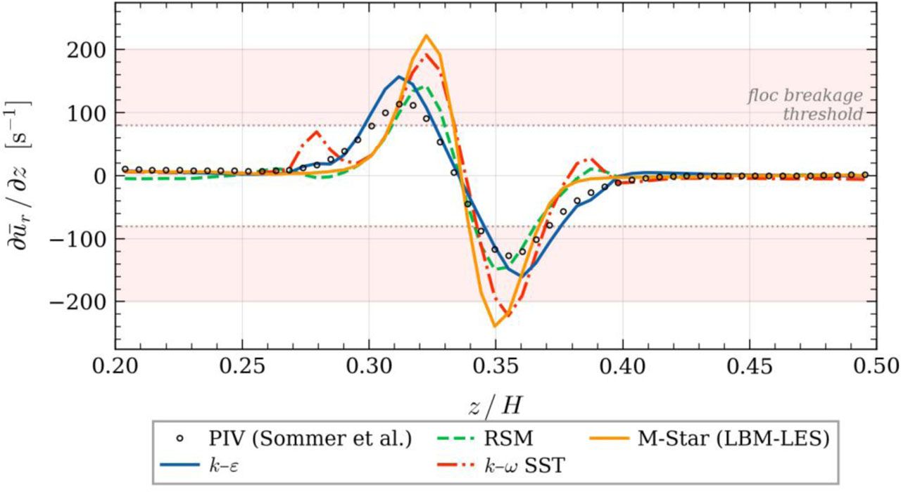
Figure 6:
Velocity gradient profiles ∂ūr/∂z [s−1] at 2r/Dt = 0.44, Ω = 650 rpm
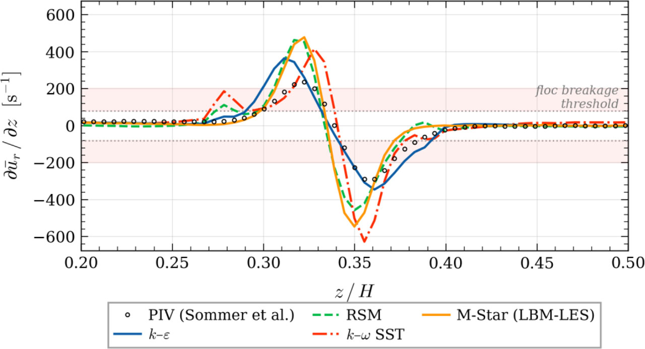
Figure 7:
Velocity gradient profiles ∂ūr/∂z [s−1] at 2r/Dt = 0.44, Ω = 1500 rpm
The velocity gradient profiles reveal the practical significance of the velocity errors. Table 3 summarizes the peak gradient magnitudes and the gradient amplification factor, defined as the ratio of the relative error in peak gradient to the relative error in peak velocity. The peak gradient according to PIV data is shown in the table for reference.
Table 3:
Peak velocity gradient magnitudes [s−1] and gradient amplification
| Condition | PIV |G|_max | k–ɛ | RSM | k–ω SST | M-Star |
|---|---|---|---|---|---|
| 650 rpm, 0.44 | 127 | 161 (+26%) | 149 (+17%) | 223 (+75%) | 239 (+88%) |
| 650 rpm, 0.80 | 30 | 31 (+3%) | 32 (+9%) | 47 (+58%) | 33 (+10%) |
| 1500 rpm, 0.44 | 289 | 364 (+26%) | 463 (+60%) | 627 (+117%) | 546 (+89%) |
| 1500 rpm, 0.80 | 85 | 68 (−20%) | 100 (+17%) | 82 (−4%) | 82 (−4%) |
At the near-impeller position (2r/Dt = 0.44), the PIV-derived peak gradient is 127 s−1 at 650 rpm and 289 s−1 at 1500 rpm. All four CFD models overestimate these peaks, with k–ω SST producing the largest gradient overshoot: 223 s−1 (+75%) at 650 rpm and 627 s−1 (+117%) at 1500 rpm. This demonstrates the gradient amplification effect: even though k–ω SST overpredicts the peak velocity by about 21% at 650 rpm, the corresponding gradient error is 75% - a roughly 3.5×amplification.
At the near-wall position (2r/Dt = 0.80), where the gradients are smaller in magnitude (30 s−1 at 650 rpm, 85 s−1 at 1500 rpm), the absolute gradient errors are smaller, but the relative amplification remains. These gradients are within the range commonly associated with floc breakage thresholds (80–200 s−1), making their accurate prediction particularly important for C&F applications.
From a practical standpoint, the spatial distributions have direct implications for estimating the volumetric fraction of the mixing vessel that exceeds the floc breakage threshold. The k–ɛ and RSM models, with their compact high-velocity cores, would predict a relatively small breakage zone confined to the immediate impeller region. The k–ω SST model, with its broader jet, would predict a larger breakage zone. The M-Star LBM-LES, with its resolved turbulent fluctuations, provides what is arguably the most physically realistic picture: a spatially heterogeneous velocity field where the transition from aggregation-favourable to breakage-prone conditions is gradual rather than abrupt, and where intermittent high-shear events can occur outside the time-averaged jet boundary. This type of information is precisely what the cumulative velocity-gradient distribution analysis advocated by (Balemans et al., 2020) requires, and it is only fully accessible through scale-resolving approaches such as LES (Figure 8).
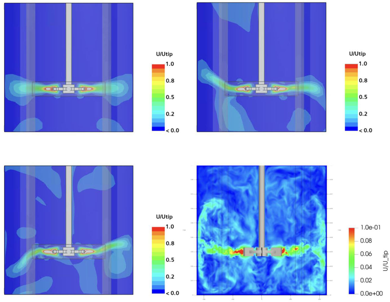
Figure 8:
Contour plots for ūr/utip in the measurement plane of the PIV dataset for k–ɛ (top-left), RSM (top-right), and k-⍵ (bottom-left) and LBM-LES models
The M-Star LBM-LES contour plot differs fundamentally from the three RANS models in its visual texture. Even after time-averaging, the velocity field retains a fine-grained spatial structure that reflects the resolved turbulent eddies. The radial jet is clearly identifiable, but its boundaries are less sharply defined than in the RANS fields – not because of excessive diffusion, but because the LES captures the intermittent, spatially varying nature of the turbulent jet. The recirculation loops show a richer internal structure with local velocity variations that are entirely smoothed out by the RANS averaging. Crucially, the M-Star contour shows a more gradual transition between the high-velocity jet core and the quiescent bulk, compared to the relatively abrupt transition in k–ɛ. This demonstrates that the LBM-LES model captures the turbulent entrainment and momentum diffusion by resolved eddies rather than imposing it through an eddy-viscosity closure.
The k–ω SST model produces the most distinctly different RANS flow field. The radial jet appears broader and more diffuse compared to k–ɛ, with the elevated-velocity region (U/utip > 0.2) extending further in the axial direction. More importantly, the recirculation pattern shows a visible asymmetry between the upper and lower loops that is less pronounced in the other RANS models. The near-wall impingement region is wider, and there are discernible patches of moderate velocity (U/utip ≈ 0.2–0.5) in the corners of the tank that are essentially absent in k–ɛ and RSM. This diffuse spreading is a direct consequence of the SST model's stress limiter, which constrains the turbulent eddy viscosity and thereby alters the jet momentum transport. The net effect is a qualitatively different spatial distribution of shear, with implications for the volumetric fraction of the tank exposed to elevated velocity gradients.
The RSM produces a velocity field that is qualitatively similar to k–ɛ but with two notable differences. First, the radial jet appears slightly narrower axially, with a more concentrated core. Second, the secondary flow features — the recirculation loops and the near-wall downward flow – are somewhat weaker than in k–ɛ, visible as a marginally smaller spatial extent of the cyan-to-green (U/utip ≈ 0.2–0.5) regions. This is consistent with the RSM's underprediction of the jet peak velocity at 650 rpm observed in the line-probe analysis (Section 3.1), which implies less total momentum in the discharge and correspondingly weaker secondary circulation.
The k–ɛ model produces the smoothest velocity field, with a well-defined radial jet that extends cleanly from the impeller tip to the tank wall. The jet core (U/utip > 0.5) is compact and axially thin, and the recirculation loops above and below the impeller plane are clearly delineated and approximately symmetric. The bulk of the vessel (outside the impeller zone and near-wall region) shows uniformly low velocities (U/utip < 0.2), indicating that k–ɛ confines the high-momentum fluid to the immediate impeller discharge. This is consistent with the model's tendency to overpredict turbulent viscosity in swirling flows, which accelerates jet decay and produces a compact high-velocity zone.
All four models correctly reproduce the principal features of the Rushton turbine flow: a strong radial jet emanating from the impeller tips at z/H ≈ 0.33, impinging on the tank wall and splitting into upper and lower recirculation loops. However, the models differ markedly in the spatial extent, intensity, and symmetry of these features.
4. Discussion
4.1. Overall Model Ranking and Turbulence Closure Performance
The results suggest a clear overall ranking: k–ɛ (0.052) > M-Star LBM-LES (0.066) > RSM (0.110) > k–ω SST (0.125); however, one should consider that it is based on axial distribution only and it should not be understood as an all-around benchmark.
The strong performance of the standard k–ɛ model is somewhat counterintuitive, given its well-documented limitations in swirling and rotating flows described in the introduction. However, this result likely reflects the specific configuration studied – a standard Rushton turbine geometry at moderate Reynolds numbers – for which the k–ɛ model's empirical constants have been extensively calibrated over decades. The model benefits from favourable error cancellation in the impeller discharge zone: its tendency to overpredict turbulent viscosity (and thus oversmooth velocity gradients) is partially compensated by the MRF approach, which artificially constrains the jet geometry.
The RSM's relatively poor performance (third overall) is noteworthy, given that it solves individual transport equations for all six Reynolds stress components. Several factors may contribute: the higher number of modelled transport equations introduces additional model constants carrying calibration uncertainty; the pressure–strain correlation model may not adequately represent the rapid distortion regime near the impeller blades; and the RSM's sensitivity to boundary conditions is generally higher than that of two-equation models. The observation that RSM switches from underprediction at 650 rpm to overprediction at 1500 rpm further suggests a Reynolds-number sensitivity in its closure.
The k–ω SST model performs worst overall, with particularly poor results at the near-wall position at 650 rpm (NRMSD = 0.213). The SST model was designed for boundary-layer flows and adverse pressure gradients (Menter, 1994), and its stress limiter, while beneficial in external aerodynamics, may over-constrain the turbulent transport in the recirculating flow of a stirred tank. The jet spreading and decay – governed by free shear rather than wall-bounded dynamics – are precisely the flow features that k–ω SST handles least well.
M-Star LBM-LES ranks second overall and shows the most spatially consistent performance: it achieves the lowest or second-lowest NRMSD at every condition except the near-impeller position, where its tendency to overpredict, peak velocity penalizes the integral error measure. Unlike the RANS models, M-Star explicitly resolves the instantaneous large-eddy structure and only models the subgrid scales via the Smagorinsky closure. The fact that its accuracy is competitive with k–ɛ – and superior to RSM and k–ω SST – at a lattice resolution of only 2403 is a practically relevant finding, as it demonstrates that GPU-accelerated LBM-LES can deliver high-fidelity velocity fields for stirred-tank geometries within feasible computational budgets. To summarize, M-Star LBM-LES allows for a great overall performance and a much better spatial distribution of turbulence quantities without requiring the computational costs of RANS models.
4.2. Gradient Amplification and Implications for Shear-Rate Estimation
The gradient analysis reveals a critically important finding for C&F applications: velocity errors are systematically amplified when converted to velocity gradients. This occurs because the gradient is a derivative quantity: even a smooth, moderate overshoot in the velocity peak translates into a steeper ascent and descent of the profile, yielding disproportionately larger gradient peaks.
The most striking example is k–ω SST at the near-impeller position: at 650 rpm, a ~21% velocity overprediction produces a ~75% gradient error (amplification factor ≈ 3.5×). At 1500 rpm, the gradient error reaches +117%, with the peak gradient (627 s−1) exceeding the PIV value (289 s−1) by more than a factor of two.
This amplification has direct consequences for flocculation modelling. If a CFD model overpredicts the local velocity gradient by a factor of two in the impeller discharge zone, the corresponding estimate of the hydrodynamic force on a floc (which scales with G or G2 depending on the breakage mechanism) will be overestimated by a factor of 2–4. In practice, this means that a designer relying on the CFD-predicted gradient field may either over-design the system by reducing impeller speed beyond what is necessary or misidentify the spatial extent of the breakage zone.
4.3. Practical Implications for Coagulation and Flocculation Design
The experimental gradients at the near-impeller position reach 127 s−1 at 650 rpm and 289 s−1 at 1500 rpm. Both values fall within or above the 80–200 s−1 range commonly reported as the transition between aggregation-dominated and breakage-dominated flocculation regimes discussed in the introduction. At the near-wall position, gradients are substantially lower (30 and 85 s−1), consistent with aggregation-favourable conditions.
This spatial heterogeneity – high gradients near the impeller, low gradients in the bulk – is precisely the type of information lost when the flow is characterized by a single global parameter. The results suggest that the choice of turbulence model matters less for predicting whether a gradient threshold will be exceeded (all models correctly identify the impeller zone as the region of highest shear) and more for predicting by how much and over what spatial extent. The latter is crucial for a proper design. For design purposes, either k–ɛ or M-Star appears suitable as a first approximation, provided the inherent uncertainty in gradient prediction (on the order of 20–75% at the impeller, depending on the model) is acknowledged. Despite limited adoption in the water sector, the LBM-LES approach appears to be a favourable choice for further investigation.
4.4. Limitations
Several limitations should be acknowledged. First, the comparison is restricted to a single velocity component (radial) at two radial positions; a complete assessment would include the axial and tangential components as well as turbulent fluctuation quantities. Second, the gradient computation relies on central finite differences applied to profiles on the PIV grid spacing; the true gradient at sub-grid scales may differ, particularly in regions of steep velocity change. Third, the M-Star simulations use a single lattice resolution (2403), and no grid-convergence study was performed for the LBM-LES results. Fourth, the study considers only steady-state (RANS) and time-averaged (LBM-LES) velocity fields; transient features such as trailing vortices and macro-instabilities are not captured by the present comparison methodology.
Finally, the experimental PIV database itself carries measurement uncertainty. (Sommer et al., 2021) report statistical uncertainties of approximately 1–3% of utip for the mean velocity fields. While this is small relative to the CFD–PIV differences discussed above, it should be kept in mind when interpreting NRMSD values below approximately 0.03–0.05, which may approach the experimental noise floor.
5. Conclusion
This study compared four turbulence modelling approaches – three finite-volume RANS closures (k–ɛ, k–ω SST, and RSM) implemented in Siemens STAR-CCM+ and one lattice-Boltzmann LES model (M-Star CFD) – against PIV-measured velocity fields in a Rushton-turbine stirred tank at two impeller speeds. The comparison was carried out on the normalized radial velocity component at two radial positions spanning the impeller discharge and near-wall regions, with accuracy quantified through NRMSD, peak velocity errors, and velocity gradient analysis.
Across all conditions, the standard k–ɛ model achieved the lowest average NRMSD (0.052), followed closely by M-Star LBM-LES (0.066), with RSM (0.110) and k–ω SST (0.125) performing substantially worse. The strong showing of k–ɛ reflects decades of calibration for this canonical geometry, while k–ω SST – designed for boundary-layer and adverse-pressure-gradient flows – proved poorly suited to the free-shear-dominated jet and recirculation of a stirred tank.
A practically important finding is the systematic amplification of velocity errors when these are converted to local velocity gradients. Moderate overpredictions of peak velocity (on the order of 20%) were shown to produce gradient errors exceeding 75%, with amplification factors of 3–4×. Since the local velocity gradient is the quantity that directly governs floc breakage and aggregation dynamics, this amplification has direct consequences for the reliability of CFD-informed flocculator design: an uncritical use of gradient fields from any RANS model may lead to substantial over- or underestimation of the spatial extent and intensity of the breakage zone.
The comparison between the RANS and LBM-LES paradigms revealed a qualitative distinction that goes beyond the scalar accuracy metrics. While k–ɛ achieved the best integral agreement with the PIV profiles, M-Star LBM-LES produced a spatially richer and physically more realistic velocity field. The contour plots showed that RANS closures yield smooth, sharply bounded jet structures, whereas the LES-resolved field retains fine-grained turbulent structure and a gradual transition between the high-shear impeller zone and the quiescent bulk. This difference is not captured by line-probe NRMSD values but is critical for applications that depend on the spatial distribution of hydrodynamic conditions – precisely the situation in coagulation and flocculation, where the volumetric fraction of the vessel exceeding a given shear threshold determines the balance between floc growth and breakage.
Indeed, the central argument of this work is that the spatial distribution of local velocity gradients – not a single global parameter such as G̅ – Is the physically meaningful basis for assessing and optimizing C&F hydrodynamics. The cumulative gradient distribution analysis advocated by (Balemans et al., 2020) demonstrated that this distribution, rather than any global or peak metric, explains flocculation outcomes that conventional parameters cannot. The present results reinforce this conclusion and add a practical dimension: the choice of CFD model determines not only the accuracy of the predicted gradient magnitudes but also the fidelity of their spatial distribution, and the two do not necessarily rank the same way.
For practitioners, these findings suggest a two-tier recommendation. For applications where scalar accuracy of the mean velocity field is the primary requirement – such as pump sizing, residence-time estimation, or preliminary design screening – the standard k–ɛ model remains a reliable and computationally economical choice. For applications where the spatial distribution of shear rates is decisive – flocculator optimization, impeller selection, or breakage-zone identification – LBM-LES offers a qualitatively superior representation of the flow, and its computational cost on modern GPU hardware is increasingly competitive. In either case, the gradient amplification effect documented here should be accounted for when translating CFD velocity fields into design criteria for mixing-sensitive processes.
Acknowledgements
This work was supported by the following funding sources: the Slovak Scientific Grant Agency under grant VEGA 1/0682/23 "Research on the interaction between surface runoff quality and groundwater quality in urbanized areas"; the Slovak Research and Development Agency under grant APVV-18-0203 “SMART management of extreme rainwater in urbanized areas”; grant VV-MVP-24-0180 “The Impact Analysis of Adaptive and Technical Measures in Urbanized Areas under Extreme Operational Conditions on Sewer Networks”; and the Grant Scheme for the Support of Excellent Teams of Young Researchers at the Slovak University of Technology in Bratislava, funded by central resources of the Rectorate of STU in Bratislava and coordinated at the Department of Sanitary and Environmental Engineering under the acronym MOZEKOV. The authors further acknowledge support from the Czech Technical University in Prague through grant SGS24/117/OHK1/3T/11 "Development of a Framework for Evaluation and Optimization of Mixing Processes during Coagulation Stage in Water and Sludge Treatment", and from the Technology Agency of the Czech Republic (TAČR) under grant SIGMA TQ03000967 "Hydraulic research of the wastewater object function".
Notes
[2] Contributed by Author Contributions
V.S. conceived and designed the study, conducted the literature research, processed the raw data, and wrote the manuscript. M.T. provided his expertise on setting up the numerical simulations and collected the data. M.P. coordinated and supervised the manuscript preparation process. Š.S. and J.P. provided expert consultations and scientific guidance. All authors critically reviewed and approved the final version of the manuscript and agreed to be accountable for all aspects of the work.