

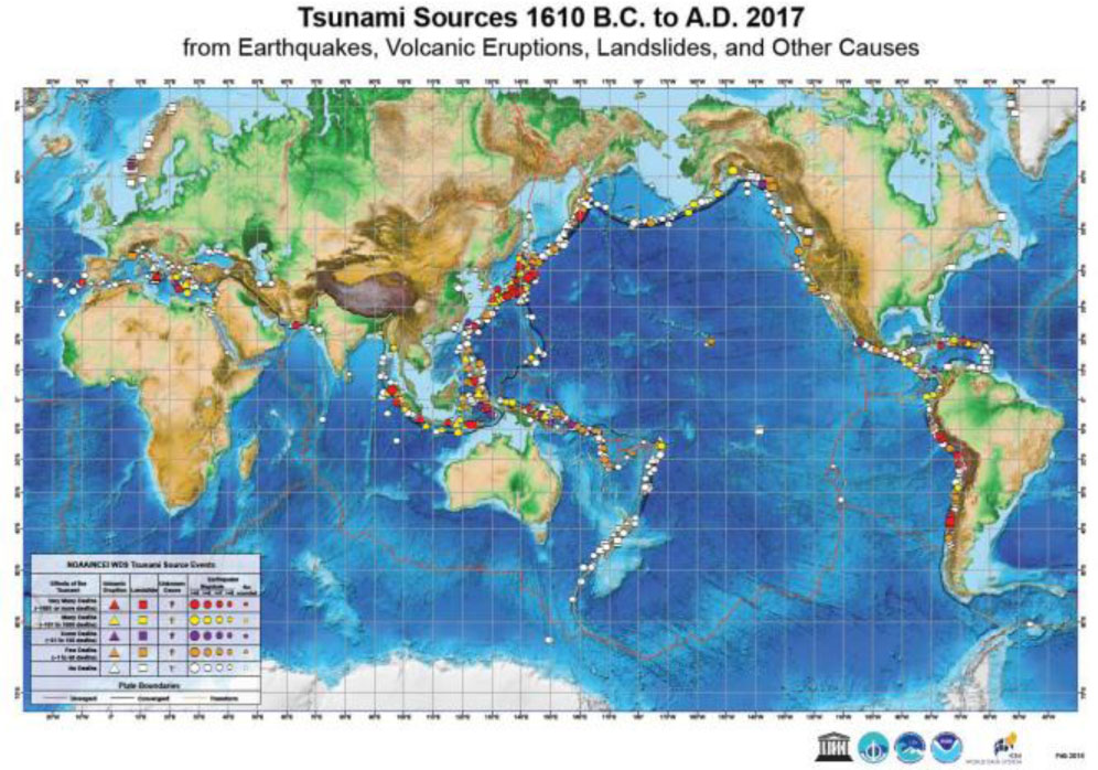
Figure 1:
Tsunami catalog (1600 BC – 2017) covering seismic, gravitational, volcanic, and other triggers. Source: NOAA
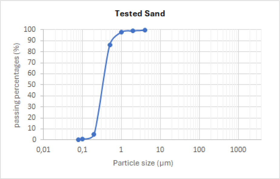
Figure 2:
Grain size distribution
Table 1:
Grading characteristics of the tested sand
| Material | D10[mm] | D30 [mm] | D60 [mm] | Cu | Cc |
|---|---|---|---|---|---|
| Sand | 0.22 | 0.29 | 0.36 | 1.64 | 1.06 |
Table 2:
Physicals properties of the tested sand
| Material | Gs | ρd min [g/cm3] | ρd max [g/cm3] | emin | emax |
|---|---|---|---|---|---|
| Sand | 2.63 | 1.44 | 1.62 | 0.419 | 0.862 |
Table 3:
Physical properties of sand vs density index
| Id | e | γd [g/cm3] | γh [g/cm3] | md [g] | mh [g] |
|---|---|---|---|---|---|
| 0.25 | 0.75 | 1.50 | 1.93 | 294.73 | 379 |
| 0.50 | 0.64 | 1.60 | 1.99 | 314.62 | 391 |
| 0.70 | 0.55 | 1.70 | 2.05 | 332.58 | 402 |
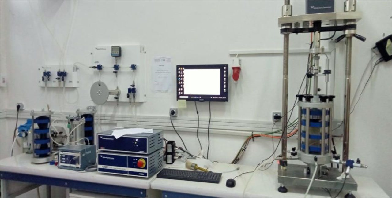
Figure 3:
The triaxial device used for monotonic and cyclic testing (DYNATIAX EmS)
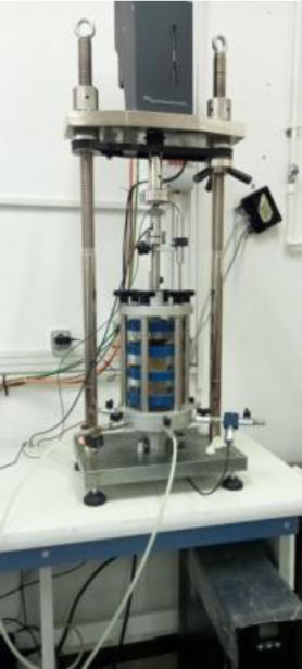
Figure 4:
Cyclic triaxial pressure cell (DYNATIAX EmS)
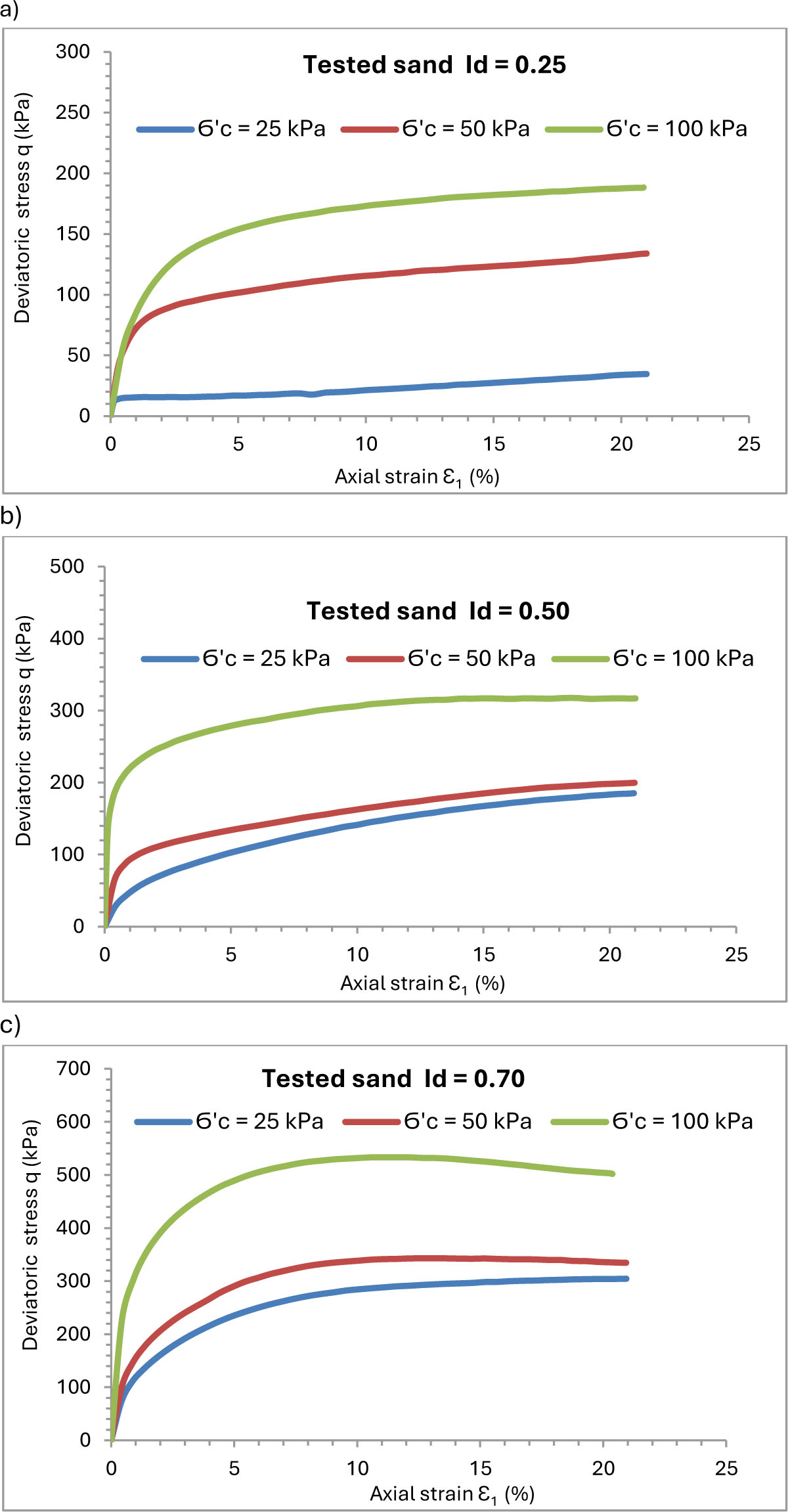
Figure 5:
Monotonic undrained triaxial compression test, stress–strain curves in the (ɛ1, q) plane a) Id = 0.25, b) Id = 0.50, c) Id = 0.70
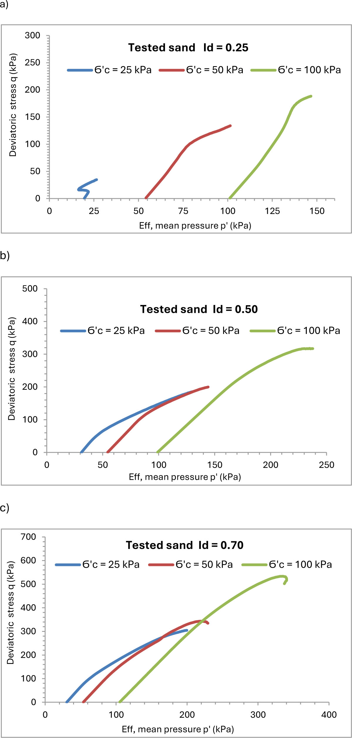
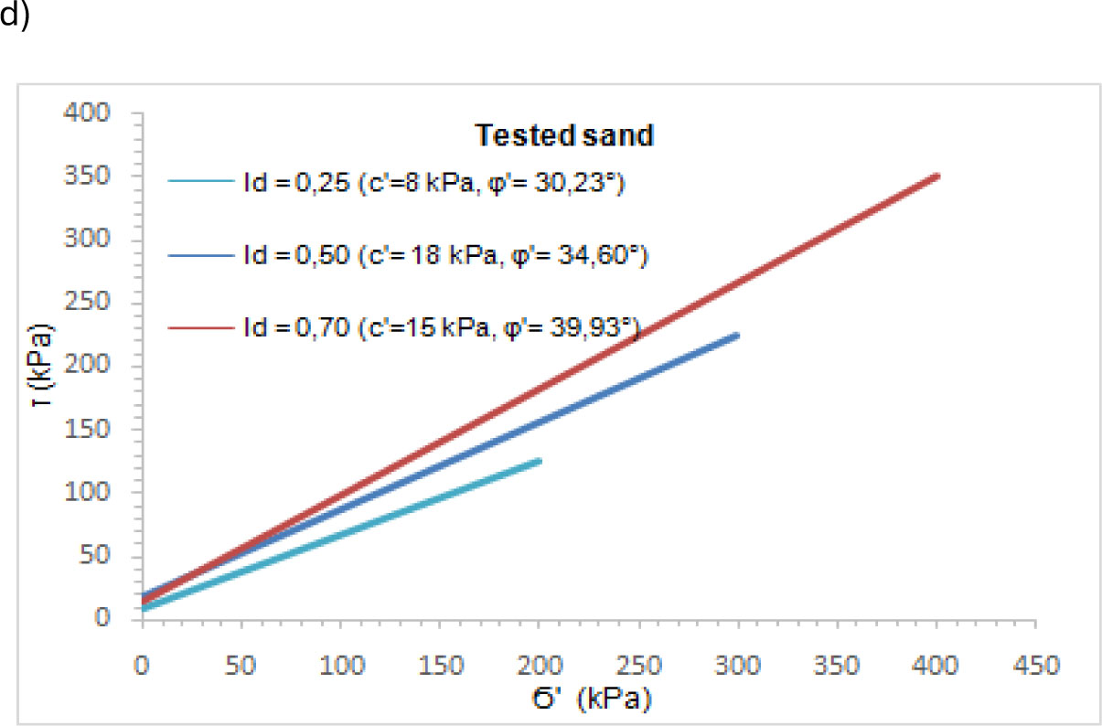
Figure 6:
Monotonic undrained triaxial compression test means effective stress–strain curves in the (p’, q) plane, a) Id = 0.25, b) Id = 0.50, c) Id = 0.70, d) The mechanical properties of the tested sand
Table 4:
Initial data for cyclic triaxial tests
| Test n° | Material | Id | Ϭc[Kpa] | F[Hz] | Amplitude [m] |
|---|---|---|---|---|---|
| 1 | Sand | 0,25 | 50 | 0,01 | 5 |
| 2 | 10 | ||||
| 3 | 0,02 | 5 | |||
| 4 | 10 | ||||
| 5 | 0,10 | 5 | |||
| 6 | 10 | ||||
| 7 | 0,50 | 0,01 | 5 | ||
| 8 | 10 | ||||
| 9 | 15 | ||||
| 10 | 0,02 | 5 | |||
| 11 | 10 | ||||
| 12 | 15 | ||||
| 13 | 0,10 | 5 | |||
| 14 | 10 | ||||
| 15 | 15 |
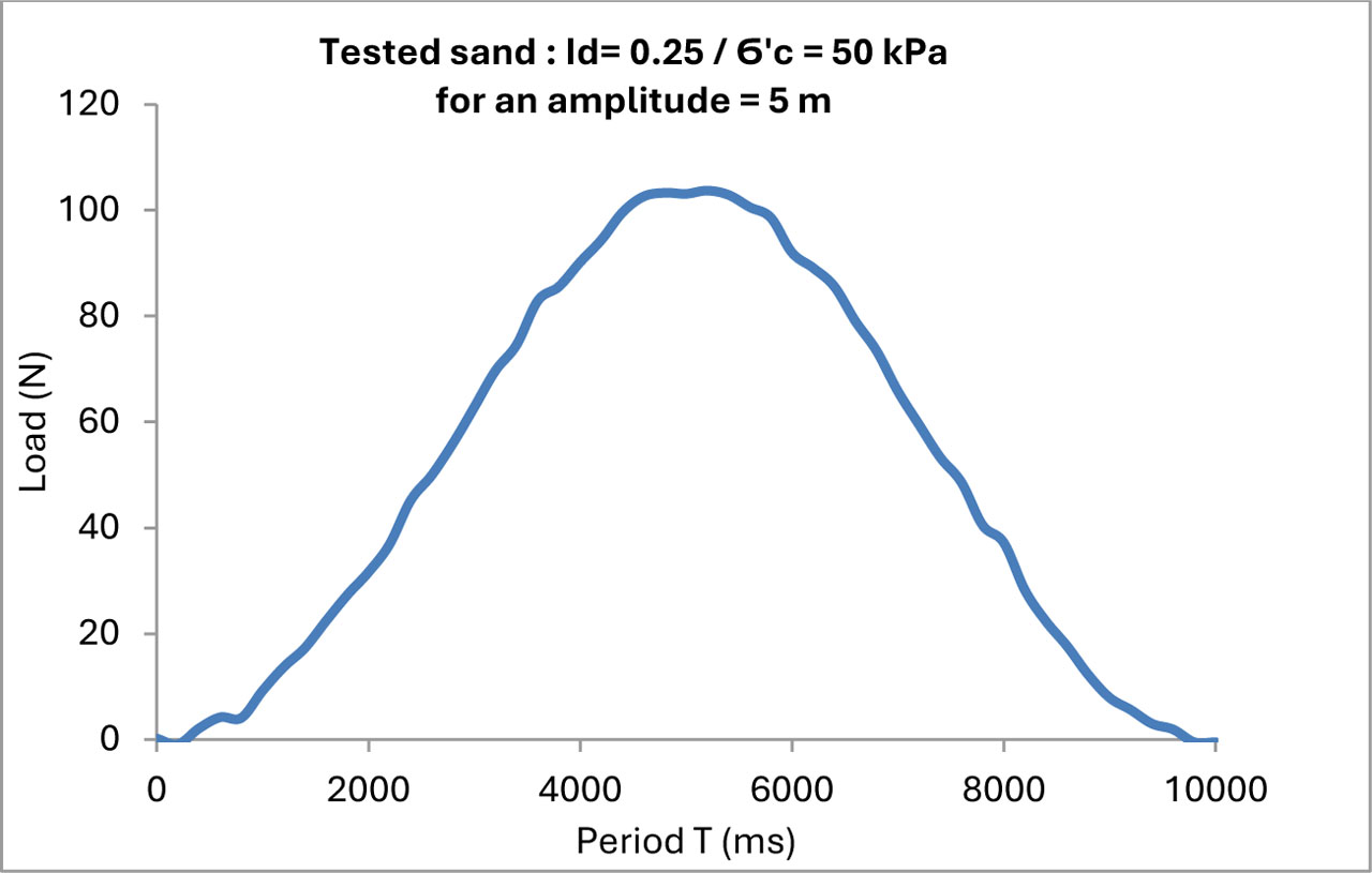
Figure 7:
Cyclic load applied to the tested sand specimen (Id=0.25, Ϭ’c=50 Kpa) during one cycle, for a 5 m wave amplitude
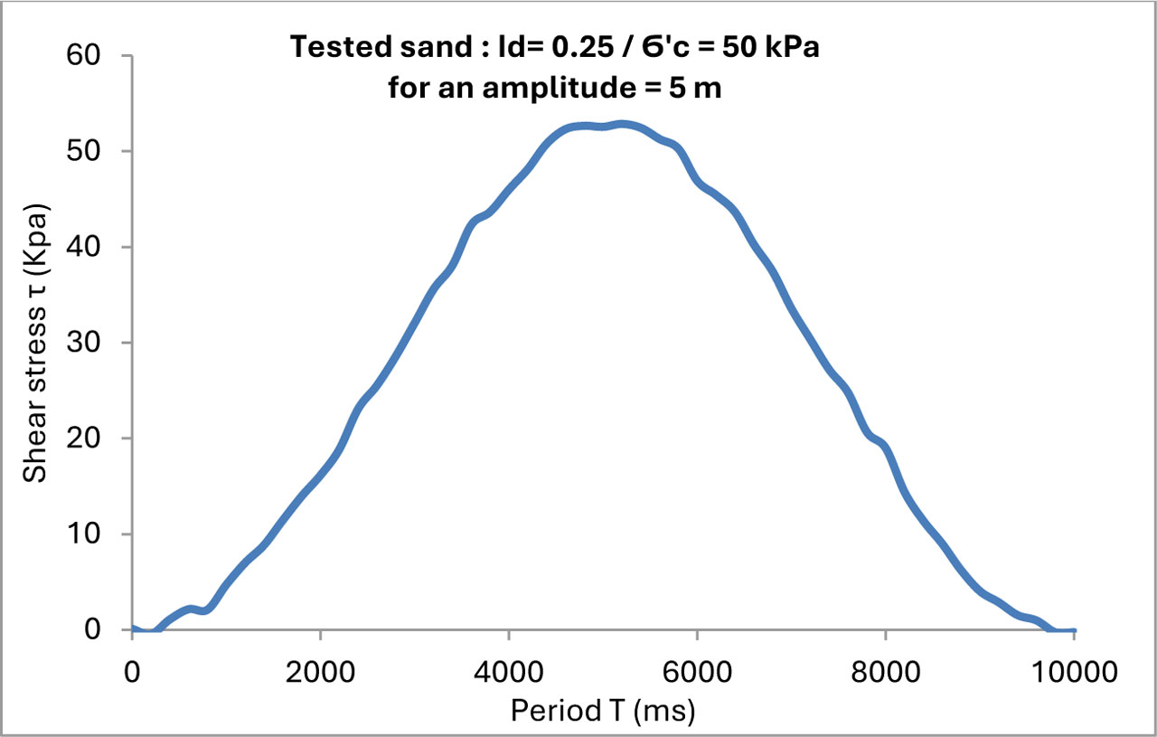
Figure 8:
Cyclic shear stress applied to the tested sand specimen (Id=0.25, σ’a = 50 Kpa) during one cycle, for a 5-meter wave amplitude
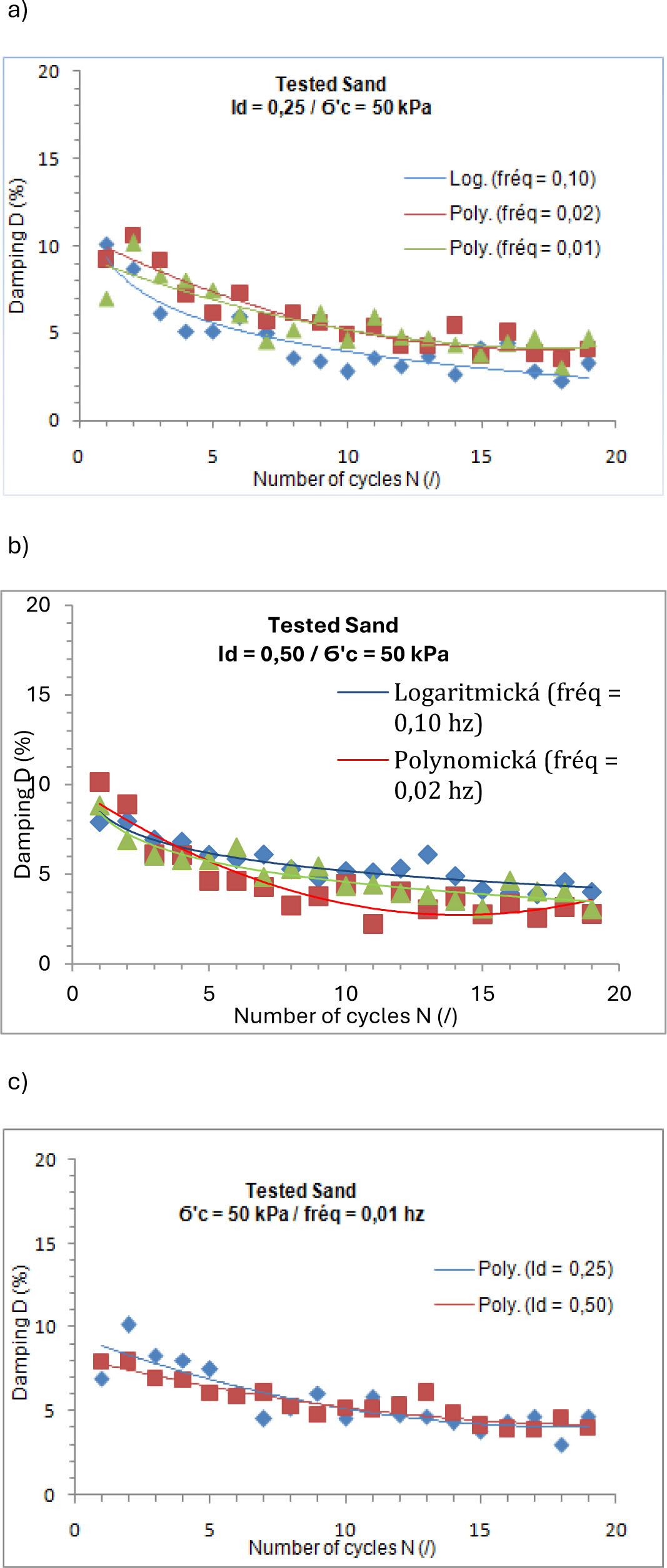
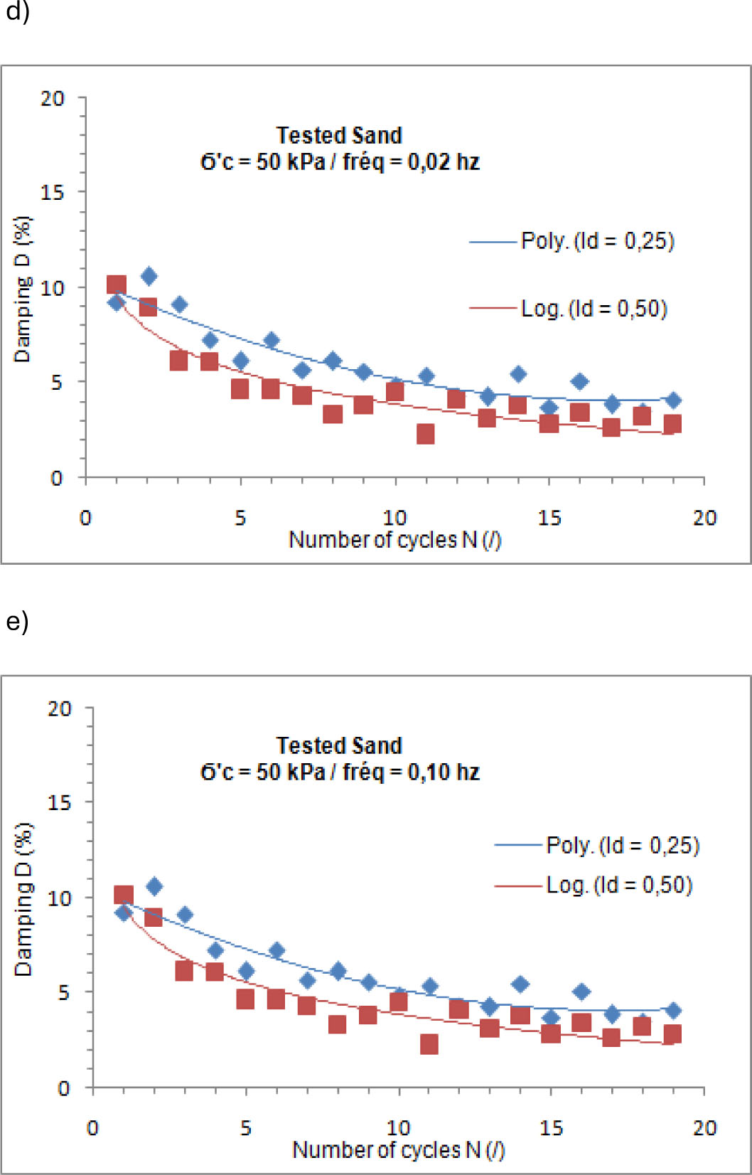
Figure 9:
Damping Ratio (D) vs. Number of Cycles Curves: a) Id = 0.25, b) Id = 0.50, c) fréq. = 0.01 Hz, d) fréq. = 0.02 Hz, e) fréq. = 0.10 Hz
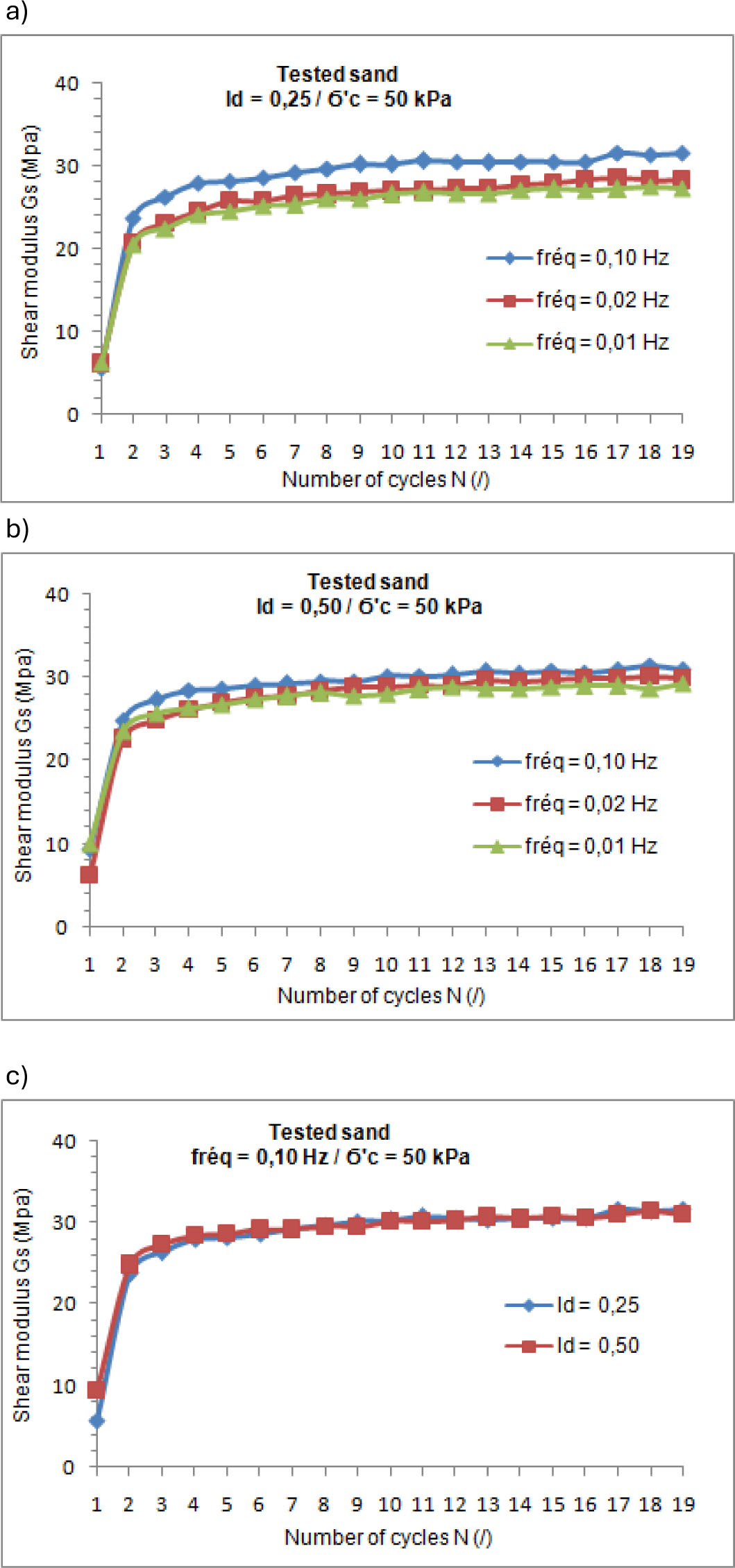
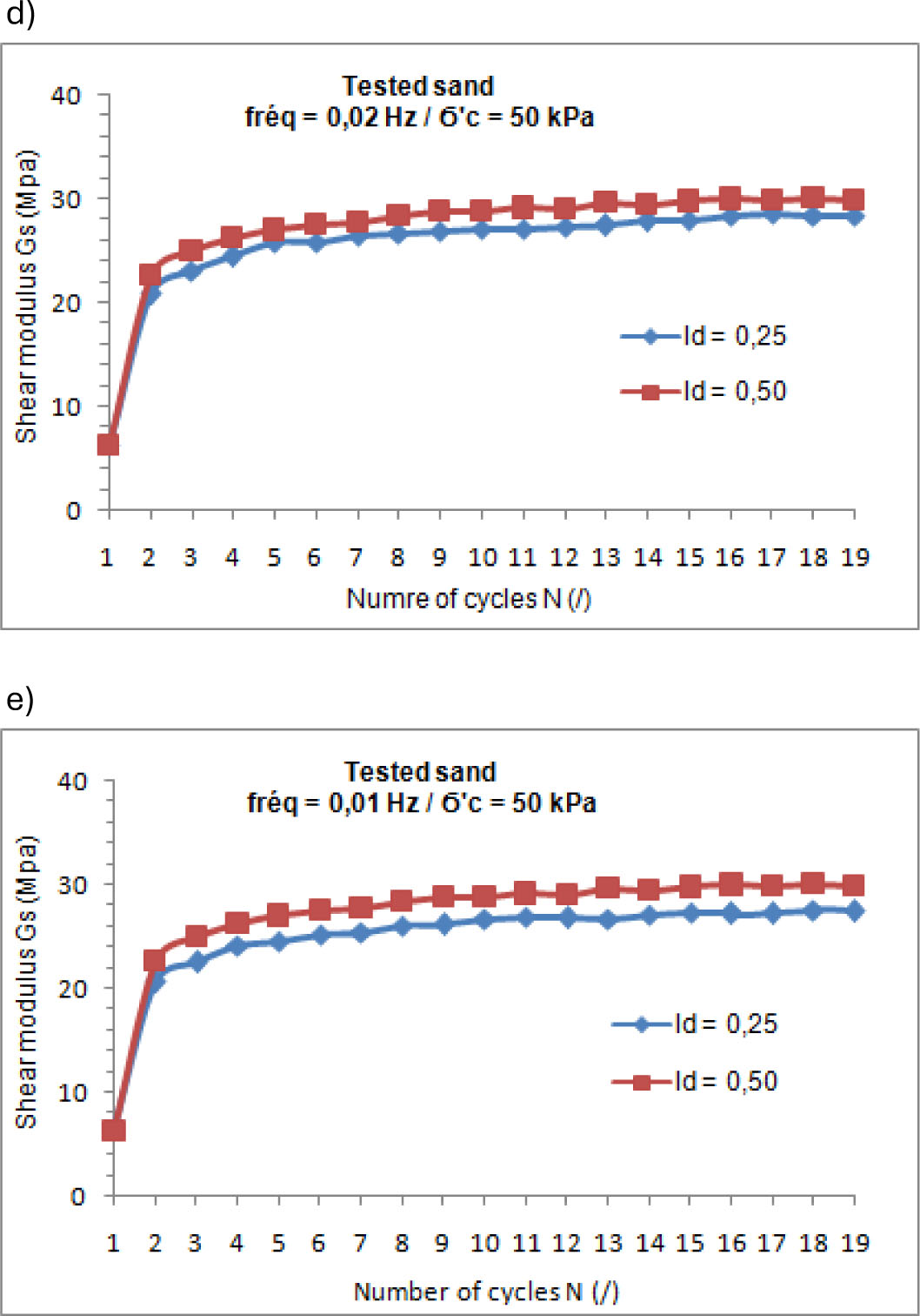
Figure 10:
Secant shear modulus (Gs) vs. Number of cycles curves: a) Id = 0.25, b) Id = 0.50, c) fréq. = 0.01 Hz, d) fréq. = 0.02 Hz, e) freq = 0.10 Hz