

1. Introduction
Among the effects induced by a major underwater earthquake are tsunamis, which are a series of enormous waves created by an underwater disturbance. Most tsunamis are of seismic origin, accounting for 81% of all generated tsunamis (National Oceanic and Atmospheric Administration, 2019). A tsunami can propagate hundreds of kilometres per hour in the open ocean and inundate land with waves reaching 30 meters or more. These are shallow-water gravity waves with periods on the order of 1,000 seconds, situated between swells (10 seconds) and tides (40,000 ± 80,000 seconds) in the ocean wave spectrum (Maria et al, 2001). As the tsunami approaches the coast, its height is approximately twice as great as at sea, and it should also be noted that its dominant wavelength becomes shorter as it nears the shore (Tatsuhiko, 2019).
Many researchers have discussed the effects of tsunamis on coastal structures. (Fritz et al, 2006) conducted an in-depth analysis of tsunami impact forces on these structures, combining laboratory experiments with theoretical discussions to better understand and assess these forces. Takahiro et al. (2014) published a summary of research on coastal structures in Tohoku, carried out at Japan’s Port and Airport Research Institute, where they interpreted damage patterns across the entire region affected by the earthquake. Their primary goal was to assess damage to coastal structures and secondary effects caused by tsunami-induced flooding. (Jayaratne et al, 2016) studied the failure modes and mechanisms of coastal structures affected by the tsunami triggered by the March 11, 2011, earthquake in northeastern Japan (Tohoku region) and provided recommendations for the design of coastal structures.
Tsunamis impact not only land-based infrastructure but also the seabed in the vicinity of ports. Research on the failure mechanisms of coastal structures damaged by tsunami-induced loads has identified foundation scour as a critical failure factor. (D.J. McGovern et al, 2019) conducted experimental research on tsunami-induced seabed erosion, demonstrating that the erosion rate is time-dependent. (Manu et al, 2023) performed a quantitative study of soil scouring phenomena beneath coastal structure foundations through rigorous numerical simulation. Their findings revealed that seabed reinforcement measures effectively reduced erosion depth by attenuating tsunami impact forces on the seabed.
The Mediterranean Sea is the world’s second most tsunamigenic zone, accounting for 15% of global events (NOAA, 2019) Figure 1. The most recent tsunami in the Mediterranean basin occurred on May 21, 2003, triggered by an Mw 6.9 earthquake off the Algerian coast. Tsunami waves reached heights of 2 m in the Balearic Islands (Spain), located 350 km northeast of the epicentral zone (Alasset and al, 2006). (Wang and Liu, 2005) studied this tsunami using numerical modelling, and the results were compared to wave heights measured in San Antonio and Ibiza (Spain). (Alasset and al, 2006) presented a study aimed at determining the tsunami source and understanding how 2 m high waves reached the Balearic Islands, while the Algerian coast was not significantly affected.
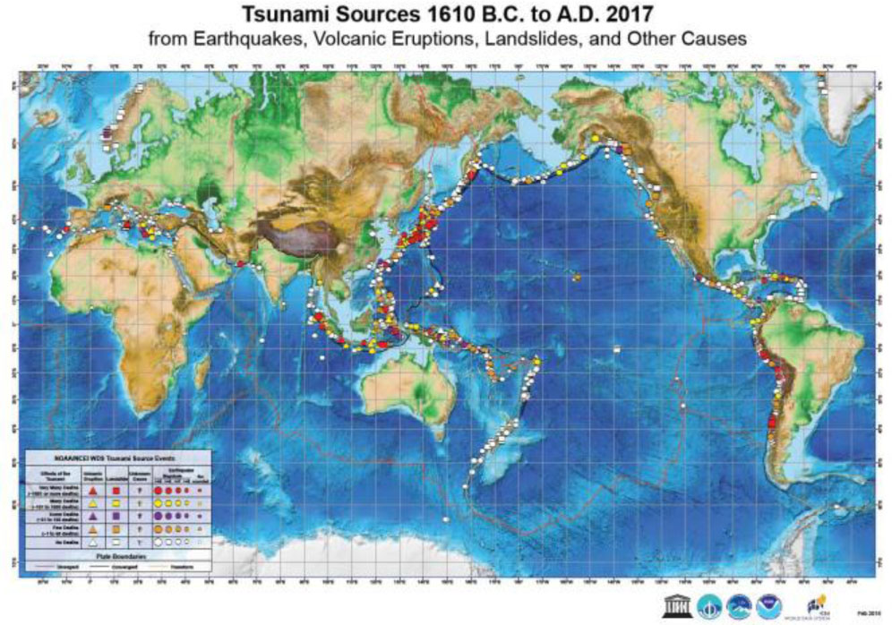
Figure 1:
Tsunami catalog (1600 BC – 2017) covering seismic, gravitational, volcanic, and other triggers. Source: NOAA
To understand the effects of tsunamis, particularly in terms of wave amplitude and frequency, on the seabed soil response in port areas, a series of dynamic behaviour characterization tests were conducted in the laboratory under various loading conditions. The tests were performed on marine soil samples collected near the new quay (Post 24) of the Port of Béjaïa, located in northeastern Algeria. Using a dynamic triaxial apparatus, the experimental setup simulated tsunami wave loading effect sunder different periods (10 s, 50 s, 100 s) and amplitudes (5 m, 10 m, 15 m). The soil specimens were prepared at two relative densities (Id = 0.25 and 0.50), in undrained conditions. The tested soil consisted of sand, whose physical and mechanical properties were characterized prior to determining its dynamic characteristics.
2. Methodology
2.1. Material
The tested material consists of sand sampled from the new quay (Post 24) at the Port of Béjaïa in northeastern Algeria. The characterization tests performed on this material included identification tests featuring grain size distribution for particles exceeding 80 micrometres in diameter, conducted according to the NF P 94-056 standard (results shown in Figure 2). The grading characteristics, including uniformity coefficient (Cu), curvature coefficient (Ce), and effective size (D10), were determined using particle diameters D30 and D60 (corresponding to 30% and 60% passing, respectively) and are summarized in Table 1. Results indicate the sand exhibits a very narrow grain size distribution. According to the Unified Soil Classification System (USCS), it is classified as poorly graded clean sand (SP). Table 2 presents the physical properties of the tested sand, including mean values of solid particle densities determined following the NF P 94-054 standard, and minimum and maximum densities determined according to the NF P 94-059 standard.
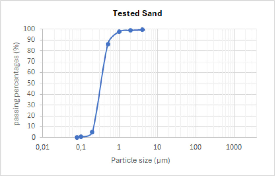
Figure 2:
Grain size distribution
2.2. Sample Preparation
The laboratory method for preparing sand samples consists of three key steps, depending on the target densities (0.25, 0.50, 0.70). In the first step: The sand sample is dried in an oven for 24 hours at 105°C. In the second step: The mass of the sample to be placed in the mold is determined based on the dry unit weight, calculated according to the void ratio and the target density. The dried and weighed sample is then lightly moistened with distilled water (5% water content) before being placed in the mold. The final stage: The specimen is prepared in accordance with ASTM D5311-92 (Reapproved 2004) using the alternative tamping compaction method. This process entails compacting the moistened sample (containing 5% distilled water) in successive layers within a membrane-lined mold, which is secured to the triaxial cell’s lower platen. The key difference from conventional compaction methods is that each layer is manually compacted using a tamping foot rather than a vibrator. It is critical to maintain constant and uniform compaction energy across each layer’s entire surface and between successive layers to ensure a homogeneous specimen. The cylindrical mold used has a diameter (D) of 50 mm and a height (h) of 100 mm. It consists of two semi-cylindrical sections that can be easily assembled or separated using clamping collars. The resulting specimen characteristics are summarized in Table 3.
2.3. Saturation
Saturation is usually accomplished by applying back pressure to the specimen’s pore water to drive air into solution, after first placing the specimen and dry drainage system under vacuum. This allows de-aired water to saturate the system while maintaining the vacuum. Among the procedures recommended by ASTM D5311-92 (Reapproved 2004) for saturation, the one starting with an initially saturated drainage system is applied: after filling the burette connected to the top of the specimen with de-aired water, a chamber pressure of 35 kPa or less is applied, and the specimen’s drainage valves are opened. Once the burette reading stabilizes, back pressure is incrementally applied to the specimen’s pore water. The specimens should be considered saturated if the B-value (Skempton’s pore pressure coefficient) is ≥ 0.95, or if the plot of B-value versus back pressure shows no further increase in B with rising back pressure. Proceed to consolidation once saturation is confirmed.
2.4. Consolidation
To achieve isotropic consolidation of the specimen, the applied back pressure must be held constant while the cell pressure is increased until the differential pressure (cell pressure minus back pressure) reaches the desired consolidation pressure. An axial load must be applied to offset the heaves induced by the rising cell pressure. This process may require incremental application of consolidation pressure to allow adequate time for applying and adjusting the compensating uplift load. Measure changes in specimen height during consolidation to the nearest 0.025 mm (0.001 in.), and the change in specimen volume to the nearest 0.1 ml.
2.5. Testing Apparatus
The setup used for both monotonic and cyclic tests is a triaxial apparatus, as illustrated in Figure 3. It consists of a triaxial pressure cell equipped with load cells, displacement transducers, and pore pressure transducers to monitor the specimen’s behaviour during cyclic loading (see Figure 4). A loading rod, connected to the upper platen through filter drains, is guided by two linear ball-bearing rings to minimize friction and maintain alignment. The loading rod seal a critical component in the cyclic soil testing cell design exerts negligible friction on the load rod. The specimen is separated from the top cap and base pedestal by rigid porous disks, which are fixed to the cap and base and have the same diameter as the specimen. The cyclic loading applied during stress-controlled cyclic triaxial tests follows a sinusoidal waveform and is conducted at different frequencies (0.01, 0.02, 0.03, and 0.10 Hz).
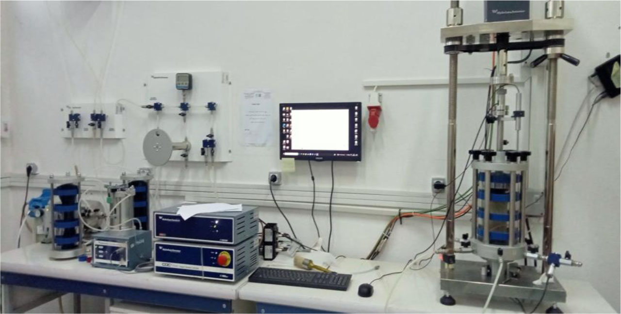
Figure 3:
The triaxial device used for monotonic and cyclic testing (DYNATIAX EmS)
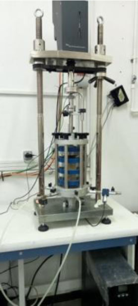
Figure 4:
Cyclic triaxial pressure cell (DYNATIAX EmS)
3. Results
3.1. Monotonic Triaxial Test Results
To complete the characterization of the sand, a triaxial test under monotonic loading in undrained compression was conducted on nine specimens. These specimens were prepared at three different densities: the first three with a density (Id = 25%), the next three with (Id = 50%), and the last three with (Id = 70%). The confining stress applied to each series of specimens with the same density was 25 kPa, 50 kPa, and 100 kPa, respectively. The test was stopped when a strain of 20% of the specimen’s initial height was reached, a threshold that had been predetermined. Figure 5 shows the stress-strain curves (ε1, q) for the three different densities: (a) Id = 0.25, (b) Id = 0.50, (c) Id = 0.70. Figure 6 presents the effective mean pressure–strain curves in the (p’, q) plane: (a) Id = 0.25, (b) Id = 0.50, (c) Id = 0.70, (d) The strength characteristics derived from the Coulomb failure line properties expressed in the (σ’, τ) plane.
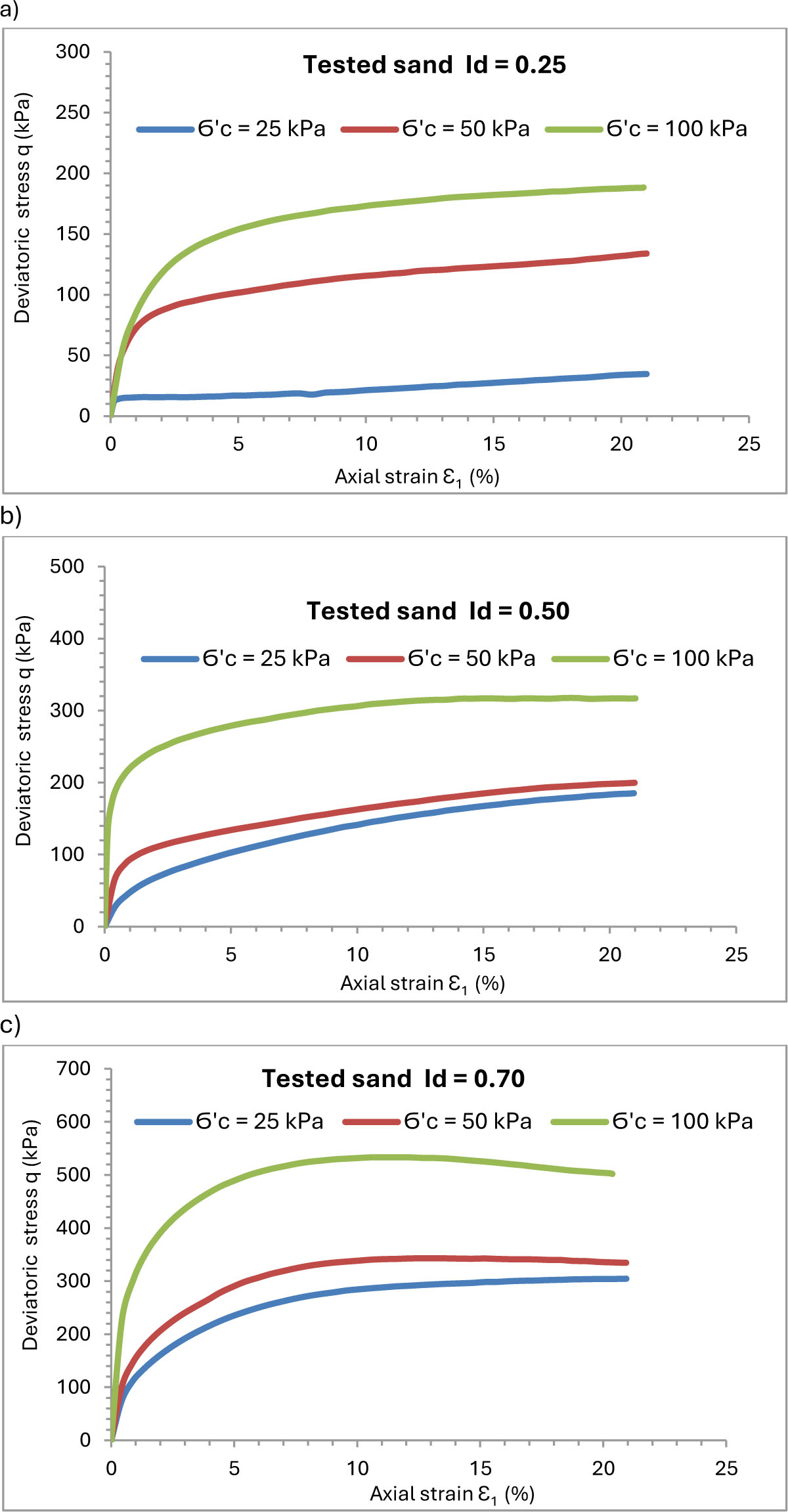
Figure 5:
Monotonic undrained triaxial compression test, stress–strain curves in the (ɛ1, q) plane a) Id = 0.25, b) Id = 0.50, c) Id = 0.70
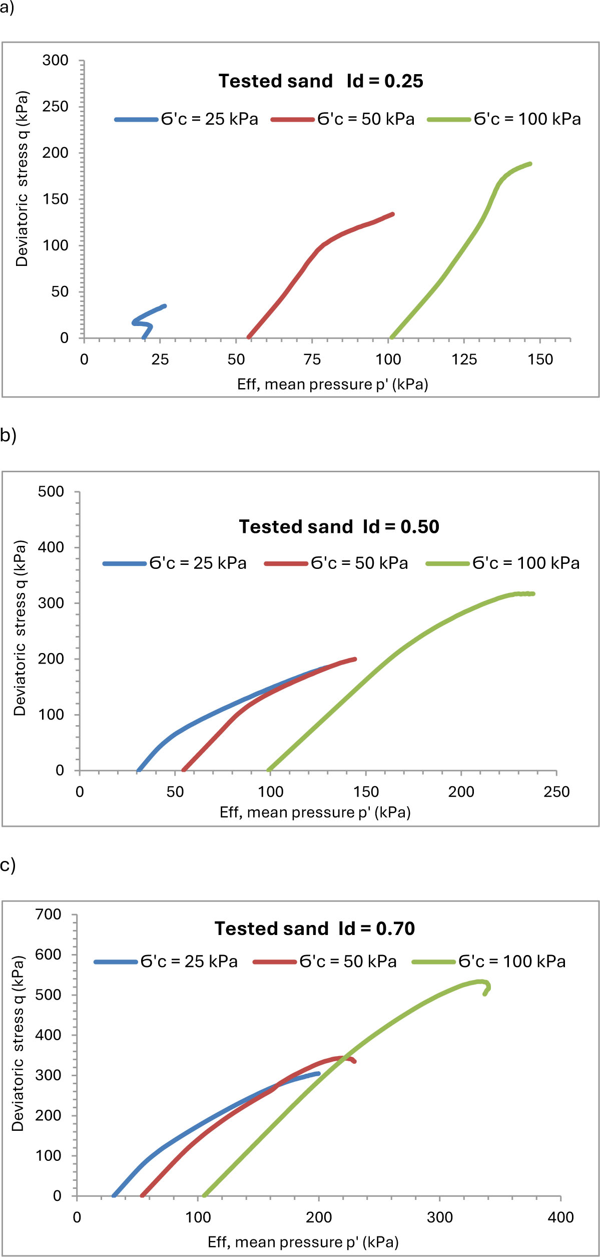
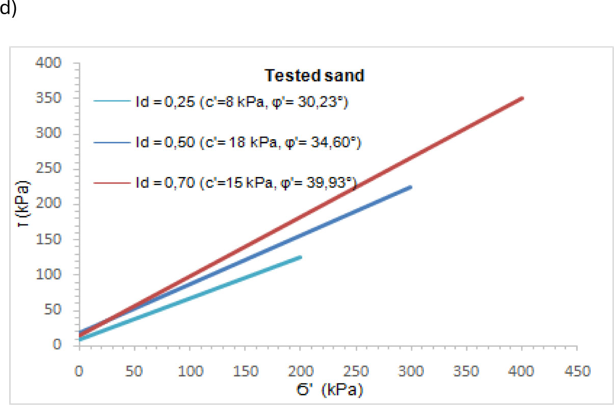
Figure 6:
Monotonic undrained triaxial compression test means effective stress–strain curves in the (p’, q) plane, a) Id = 0.25, b) Id = 0.50, c) Id = 0.70, d) The mechanical properties of the tested sand
3.2. Cyclic Triaxial Test Results
Two series of stress-controlled cyclic triaxial tests under undrained conditions were conducted on a total of fifteen specimens. The first series, consisting of six specimens, was prepared at a relative density (Id = 0.25) and a confining pressure of 50 kPa. For this series, we experimentally simulated the effects of a tsunami-like wave load with different periods (10 s, 50 s, 100 s) and amplitudes (5 m, 10 m). The second series, comprising nine specimens, was prepared at a higher relative density (Id = 0.50) while maintaining the same confining pressure (50 kPa). In this case, we also replicated tsunami wave loading effects, but with a broader range of periods (10 s, 50 s, 100 s) and amplitudes (5 m, 10 m, 15 m). Table 4 summarizes the initial test parameters for the cyclic triaxial tests.
Table 4:
Initial data for cyclic triaxial tests
| Test n° | Material | Id | Ϭc[Kpa] | F[Hz] | Amplitude [m] |
|---|---|---|---|---|---|
| 1 | Sand | 0,25 | 50 | 0,01 | 5 |
| 2 | 10 | ||||
| 3 | 0,02 | 5 | |||
| 4 | 10 | ||||
| 5 | 0,10 | 5 | |||
| 6 | 10 | ||||
| 7 | 0,50 | 0,01 | 5 | ||
| 8 | 10 | ||||
| 9 | 15 | ||||
| 10 | 0,02 | 5 | |||
| 11 | 10 | ||||
| 12 | 15 | ||||
| 13 | 0,10 | 5 | |||
| 14 | 10 | ||||
| 15 | 15 |
3.2.1. Cyclic Loading
The translation of tsunami characteristics (wave height, period) into cyclic stress parameters in a triaxial test is a multi-step process:
Step1: The tsunami wave height (H) is not directly applied as a stress amplitude in the test. It is first converted into an additional hydrostatic pressure exerted on the seabed. This pressure (p) is calculated according to the fundamental principle of hydrostatics:
where :ρ - is the density of seawater (≈ 1025 kg/m3),
g - is the acceleration due to gravity (9.81 m/s2),
H - is the tsunami wave height (m).
For example, a 5 m high wave generates a maximum bottom pressure of:
P = 1025 × 9.81 × 5 ≈ 50,276 Pa = 50 kPa.
This value represents the maximum increase in total vertical stress due to the passage of the wave.
Instead of applying a water pressure, a cyclic axial force is applied as shown below.
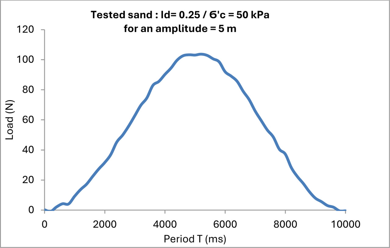
Figure 7:
Cyclic load applied to the tested sand specimen (Id=0.25, Ϭ’c=50 Kpa) during one cycle, for a 5 m wave amplitude
Step2: In a cyclic triaxial apparatus, the water pressure is not directly replicated; instead, the variation in shear stress is reproduced. The passage of the waves creates a cyclic shear solicitation within the soil. The cyclic shear stress (τcyc) is defined as half the difference between the maximum and minimum total stresses applied during a cycle, as represented below.
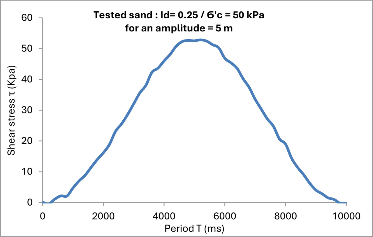
Figure 8:
Cyclic shear stress applied to the tested sand specimen (Id=0.25, σ’a = 50 Kpa) during one cycle, for a 5-meter wave amplitude
Step 3: The experimental protocol for the cyclic apparatus is therefore determined as follows:
○ Application of Cyclic Loading: Instead of applying a water pressure, a cyclic axial force is applied. The amplitude of the cyclic deviatoric stress (qcyc or σdcyc) is determined in Step 2.
○ Frequency: The loading frequency is selected to be representative of the tsunami wave period. A higher frequency simulates the more rapid loading occurring near the coast.
4. Discussion
4.1. Evolution of Damping in Tested Sand with Number of Cycles
The diagrams in Figure 9 (a) and (b) show the evolution of damping in sand with variable density under different frequencies as a function of the number of cycles. The following observations are made:
○ For sand with a density (Id = 0.25): The damping (D) decreases rapidly up to the 5th cycle, while beyond the 5th cycle, the decrease is slower, stabilizing around the 15th cycle. The damping rates are nearly identical and coincide for frequencies of 0.01 and 0.02 Hz, whereas for the higher frequency of 0.10 Hz, the damping values are significantly lower than those at 0.01 and 0.02 Hz.
○ For sand with a density (Id = 0.50): The damping decreases rapidly up to the 5th cycle, where the values for frequencies of 0.01, 0.02, and 0.10 Hz nearly coincide. Beyond the 5th cycle, the damping tends to stabilize.
The diagrams in Figure 9 (c), (d), (e) illustrate the evolution of sand damping for different densities (0.25 and 0.50) under a fixed confining stress of 50 kPa and at frequencies of 0.01, 0.02, and 0.10 Hz. The following observations are noted:
○ At a frequency of 0.01 Hz: The damping ratio decreases similarly regardless of sand density (Id = 0.25 or 0.50), with nearly coinciding values.
○ At frequencies of 0.02 and 0.10 Hz: A rapid decrease is observed up to the 5th cycle, after which the values tend to stabilize. For these frequencies, sand with a density of 0.25 exhibits higher damping ratios compared to sand with a density of 0.50.
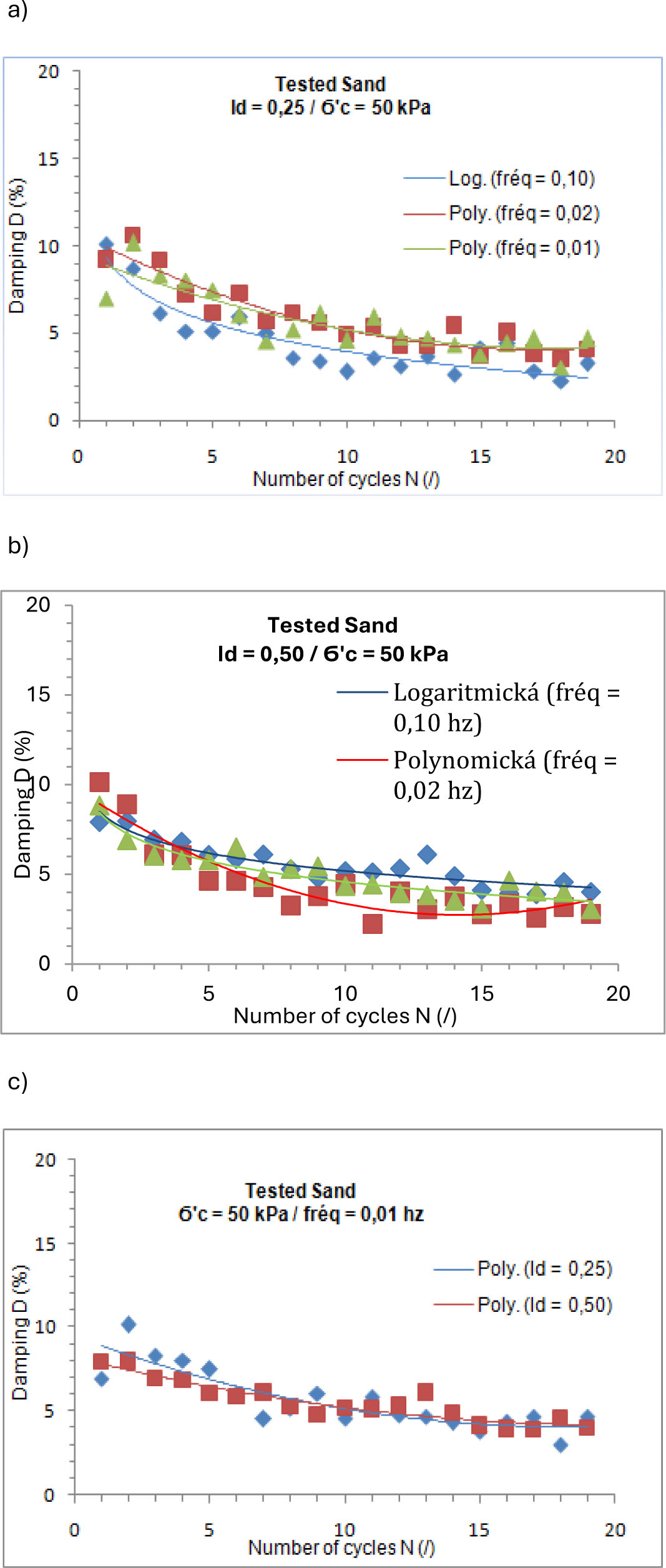
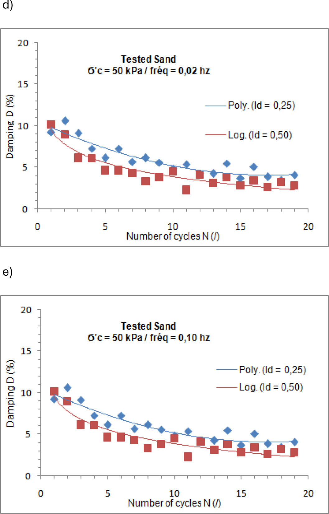
Figure 9:
Damping Ratio (D) vs. Number of Cycles Curves: a) Id = 0.25, b) Id = 0.50, c) fréq. = 0.01 Hz, d) fréq. = 0.02 Hz, e) fréq. = 0.10 Hz
4.2. Effect of Loading Frequency on Tested Sand Behaviour
Figure 10 (a) and (b) present the evolution of the secant shear modulus (Gs) as a function of the number of cycles for different loading frequencies (0.01, 0.02, and 0.10 Hz). The following trends are observed:
○ For sand with a density (Id = 0.25): The secant shear modulus (Gs) evolves rapidly up to the 2nd cycle, then progresses slowly between the 2nd and 5th cycles, before stabilizing beyond the 5th cycle. (Gs) increases with frequency, with nearly identical values at 0.01 and 0.02 Hz, at 0.10 Hz, (Gs) shows as light increase compared to 0.01 and 0.02 Hz.
○ For sand with a density (Id = 0.50): The evolution of Gs follows a similar trend to that of the lower-density sand (Id = 0.25). However, the effect of loading frequencies (0.01, 0.02, and 0.10 Hz) on (Gs) variation is almost negligible.
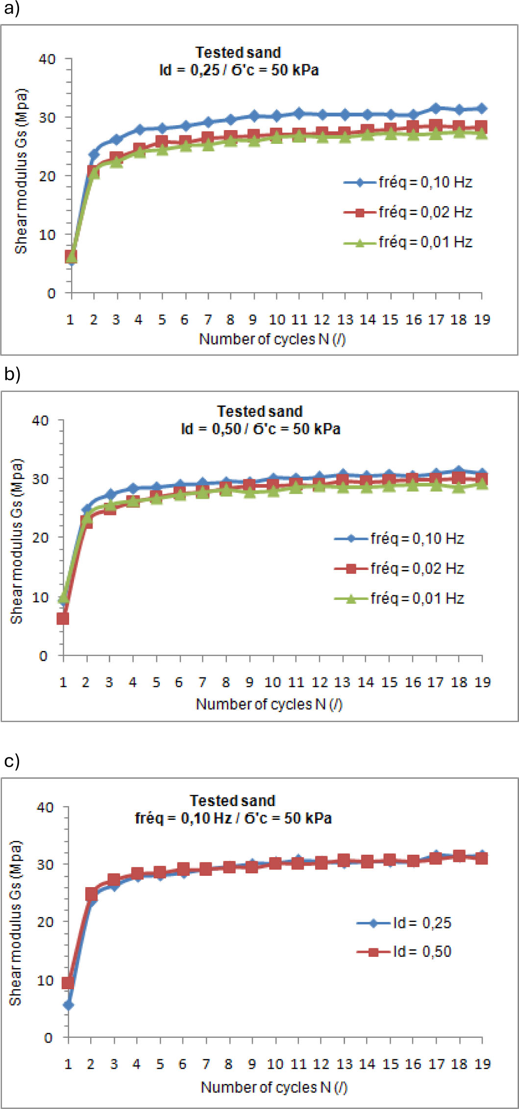
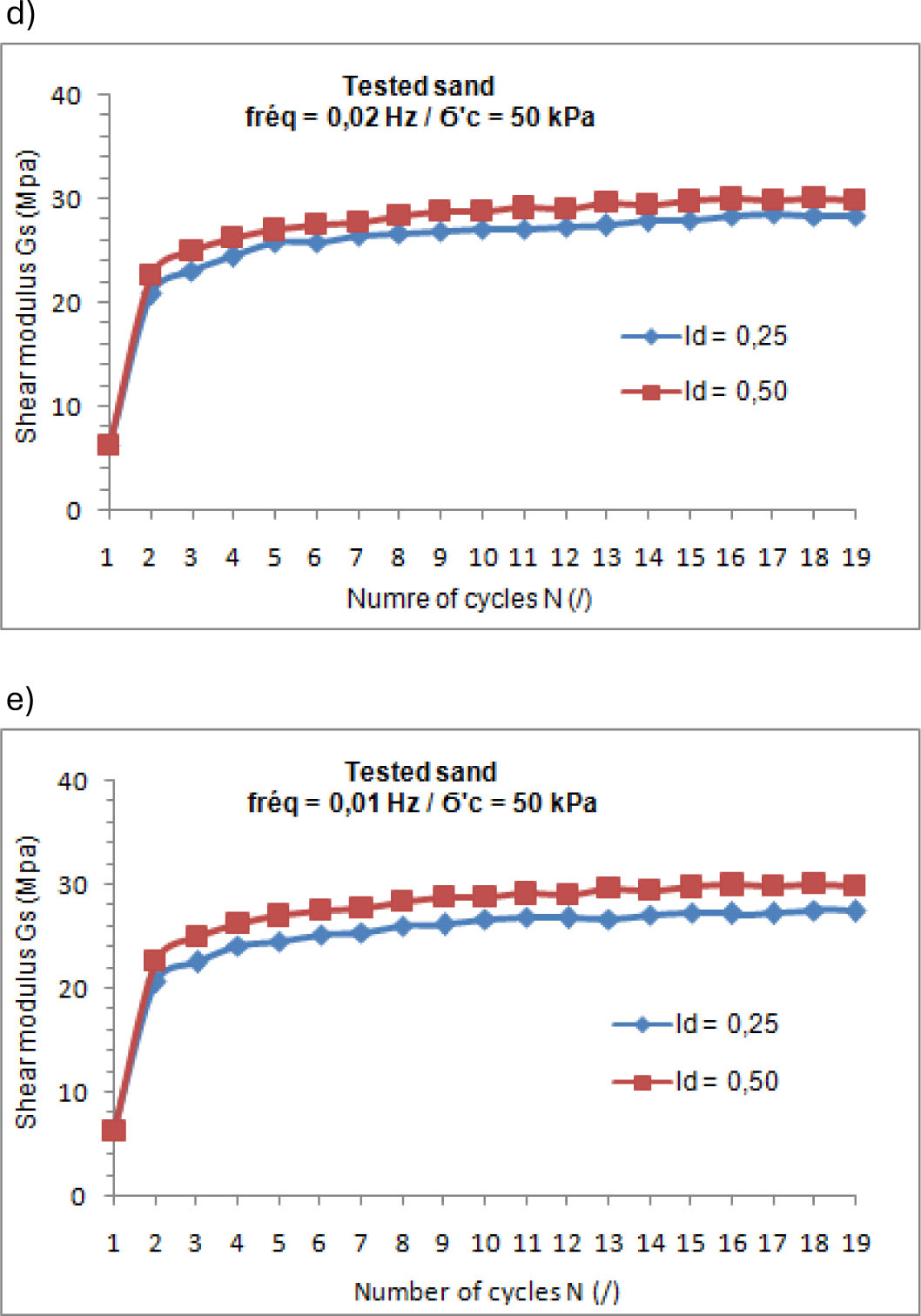
Figure 10:
Secant shear modulus (Gs) vs. Number of cycles curves: a) Id = 0.25, b) Id = 0.50, c) fréq. = 0.01 Hz, d) fréq. = 0.02 Hz, e) freq = 0.10 Hz
Figure 10 (c), (d), (e) illustrate the evolution of Gs as a function of the number of cycles for two relative sand densities (Id = 0.25 and 0.50). The analysis reveals the following:
○ At 0.01 Hz, sand with (Id = 0.50) exhibits higher (Gs) values than sand with Id = 0.25. As the frequency increases (from 0.01 to 0.02 Hz and up to 0.10 Hz), this difference gradually diminishes, becoming negligible at higher frequencies.
It is noted that:
○ The secant shear modulus (Gs) is significantly influenced by frequency for sand with a density of (Id = 0.25), whereas sand with a density of (Id = 0.50) exhibit slow sensitivity to frequency variations.
The effect of density on the dynamic behaviour of the tested sand is more pronounced at low frequency (0.01 Hz) but becomes negligible at high frequency (0.10 Hz).
5. Conclusion
Undrained cyclic triaxial tests were carried out on fifteen specimens of marine sand, sampled near the new quay of the port of Béjaïa (Algeria). The objective was to study its dynamic behaviour under loadings similar to those induced by tsunami waves. The specimens, prepared with two relative densities (Id = 0.25 and 0.50), were subjected to different frequencies (0.01, 0.02 and 0.10 Hz) and loading amplitudes (5, 10 and 15 m), under a constant confining pressure (σ’c = 50 kPa). The main results of this experimental study are as follows:
○ Energy Dissipation: For loose sand (Id = 0.25), energy dissipation is strongly influenced by frequency. It is higher at low frequencies (0.01 – 0.02 Hz) and decreases significantly at the higher frequency (0.10 Hz). Furthermore, it decreases with the number of loading cycles.
○ Stiffness Evolution: The stiffness of the sand increases rapidly during the initial loading phase, then its rate of increase slows down before stabilizing. This trend is observed for both loose and dense sand.
○ Influence of Frequency on Stiffness: The stiffness of medium to high-density sand (Id = 0.50) is weakly dependent on the loading frequency (between 0.01 and 0.10 Hz). In contrast, the stiffness of loose sand is much more sensitive to it.
○ Predominant Role of Density: The initial density state of the sand is a crucial parameter for its cyclic behavior, particularly under low frequencies (0.01 Hz). In contrast, its influence becomes negligible under high-frequency loading (0.10 Hz).
It should be noted that the conclusions of this study are drawn from laboratory experiments conducted with a dynamic triaxial apparatus under specific conditions. Actual field conditions are naturally more complex. Nevertheless, the results under controlled conditions reveal significant trends. They demonstrate that the seabed soil’s response to tsunami-type cyclic loading is strongly influenced by its density and the frequency of the applied loading. Under rapid cyclic loading (high frequency, e. g, 0.1 Hz), Loose sand (low density) exhibits lower energy dissipation and a greater amplification of effects, making it highly vulnerable. In contrast, dense sand effectively attenuates these effects. Under slow cyclic loading (low frequency, e. g, 0.01–0.02 Hz), The behaviour of the sand becomes much less sensitive to variations in density. The effects are similar, whether the soil is loose or dense.
Thus, the characteristics of the tsunami loading, particularly its frequency and amplitude, are key parameters for assessing the risk of seabed soil degradation, in interaction with its density.
Acknowledgements
This study received financial support from the Directorate of Doctoral Training, Ministry of Higher Education and Scientific Research of Algeria (PRFU Project, number: A01L02UN410120220001).