

Thermal cameras detect infrared radiation and convert the collected data into visual images. Professional cameras collect radiometric data for each pixel recorded by the sensor and this data can be accessed by the user. But there are also many types of thermal cameras that can’t deliver the temperature data and can display only a legend about the correspondence between the gray levels and the extreme temperatures of the image. The proposed method performs this conversion from grayscale values to temperature data with high accuracy, using the recordings from a FLIR A700 infrared (IR) camera. This camera returns grayscale images with legend for temperature but also a file with the temperatures recorded by the sensors; the data from this file will be used as a reference to calculate the conversion error.
Infrared thermography has been used increasingly often in industrial and military applications as shown in the reviews of Osornio-Rios, Antonino-Daviu and Romero-Troncoso (2019), Venegas, Ivorra, Ortega and Sáez de Ocáriz (2022), or the analysis of dosimetry measurements by Neghină, Cotoi, Voina and Miclăuş (2022). Because the technical characteristics of thermal cameras change and improve constantly, the necessity of accurate conversions from grayscale levels to temperatures remains an active research topic, independent of geometric camera calibration, as discussed in ElSheikh, Abu-Nabah, Hamdan and Tian (2023), self-radiance control as in Dong, Huang, Yan and Jiang (2013) or the study of external effects related to the environment, as discussed by Vendt et al. (2011) or the thermal emissivity of various materials, as in Li, Tian and Ahmed (2023). In situations where the camera only outputs an image (with the corresponding temperature scale embedded rather than included separately), or the file containing the temperature values is lost or corrupted, the conversion can only be achieved through image processing techniques.
Regression models are the most straightforward technique of converting temperature directly from grayscale intensity values. Chen and Kuo (2015) studied the conversion under the assumption that the image acquisition process may have been corrupted and the grayscale levels may have been affected by (white) noise, thus considering a second degree polynomial curve fitting. However, even in the absence of image noise, there is still the problem of correctly identifying the temperature range of the grayscale levels from potentially unreliable labels and then scaling the temperatures accordingly.
Infrared thermal images were extracted from a video recorded with a FLIR infrared camera, with a framerate of 1Hz and a resolution of 480 x 640 px, for a duration of approximately 20 minutes (more exactly, 1158 frames). Each IR image has a legend as in Figure no. 1, which contains 2 boxes with the minimum and the maximum temperature from the image and 13 intermediate points indicating levels of gray between black and white. Using the FLIR Research Studio Software, the thermal images of the frames were converted to absolute temperature values and exported as *. csv files. The information from the csv file will be used as reference.
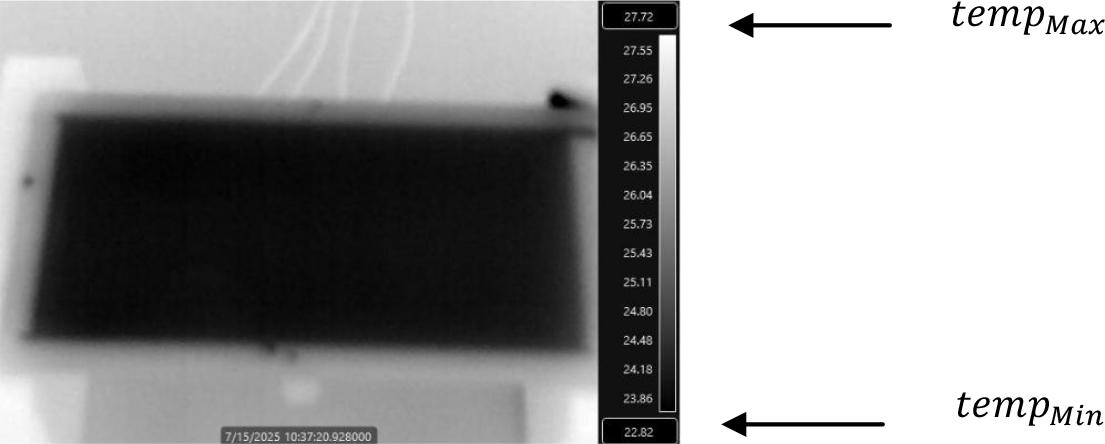
The infrared image with the legend of temperature
(Source: Matlab simulation)
In order to transform each grayscale image into a map of temperatures, it is necessary to determine the minimum and the maximum temperature from each frame. This operation was performed by two methods: a) Method 1: extracting the extreme temperatures directly from the legend of each frame; b) Method 2: extracting all the 13 intermediate points from the legend of each frame, determine the regression line and estimating the minimum and maximum values of the temperature. Knowing the extreme temperatures for each frame, a linear conversion between the intensity of the pixel and the temperature value was realized as in chapter 3.2.
From each frame, the extreme temperatures of the legend were extracted using the Tesseract OCR engine described in Smith R. (2007) to perform automatic text detection and recognition. Because the legend of the infrared image (the temperature scale) is always at the same coordinates, predefined areas of 20 x 50 px were used to search for the minimum and maximum values in order to increase the accuracy and speed of the OCR algorithm. The accuracy of automatic reading from the legend of minimum and maximum temperature using OCR was 100%.
In Figure no. 1, the maximum value tempmax corresponds to the brighter pixel and the minimum value tempMin corresponds to the darker pixel from the image.
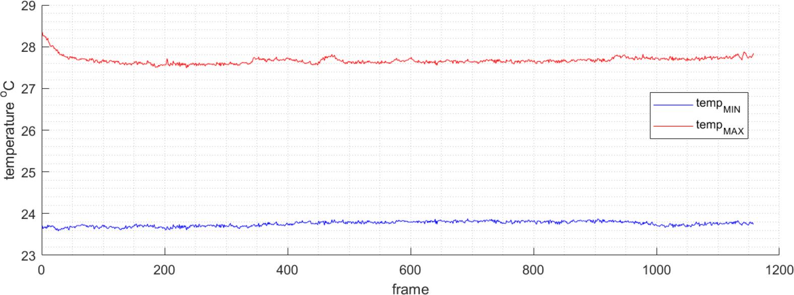
Figure no. 2 shows the temporal evolution of the minimum and maximum temperature values across all frames, extracted from the IR image legend using OCR. Although all extreme temperatures were correctly identified automatically from the legend, there are some spikes in the evolution of the minimum temperature (as can be seen in Figure no. 2.a), which seem unnatural and most likely appear when the camera updates its temperature range for individual frames. These spikes can be easily filtered out with a median linear filter of length 3 with the results in Figure no. 2.b.
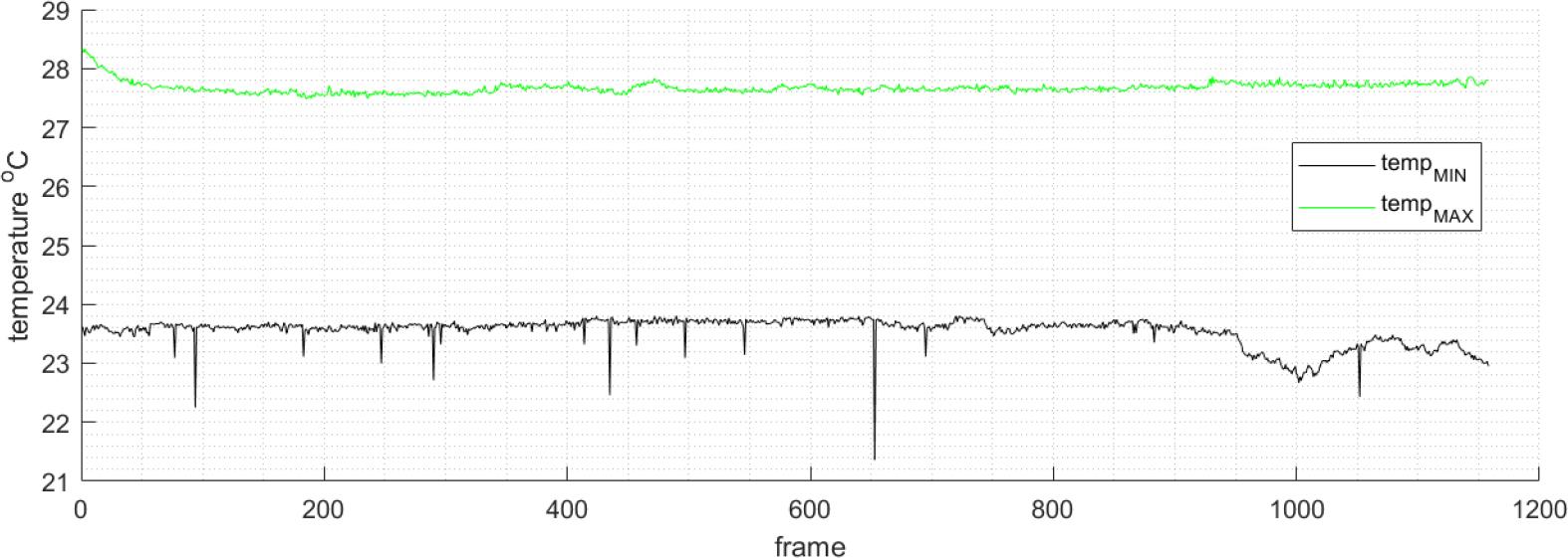
The evolution of the minimum and maximum temperature values
(Source: Matlab simulation)
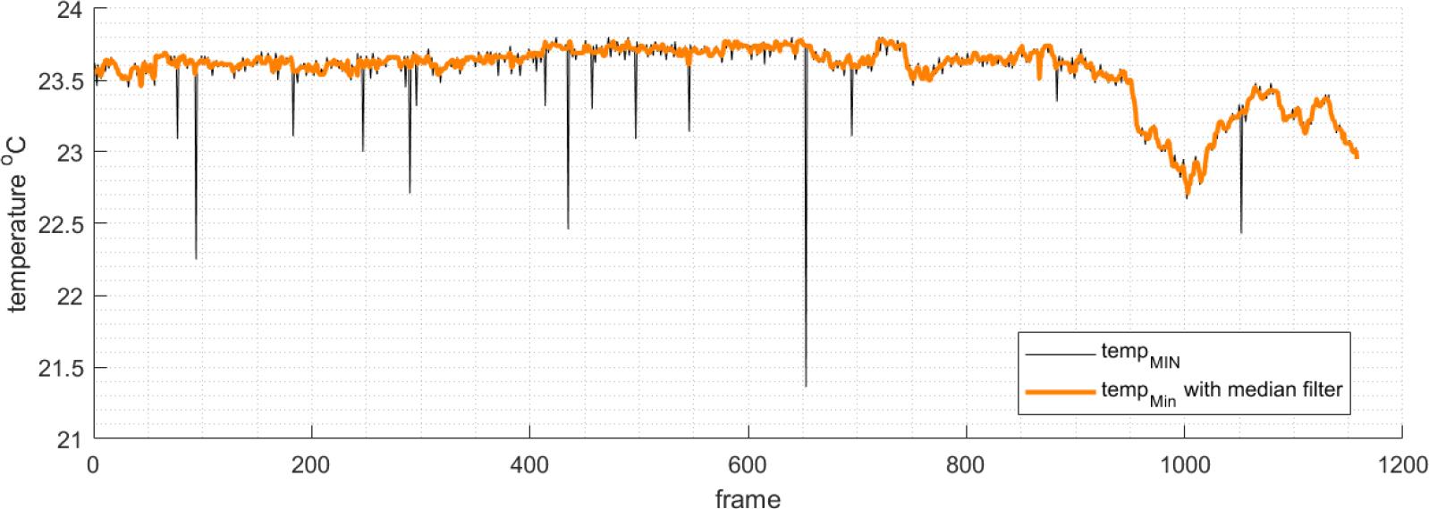
The evolution of the minimum temperature values without and with median filter
(Source: Matlab simulation)
The idea of this method is to estimate the minimum and maximum temperature from each frame using only the 13 intermediate points from the legend and linear regression. As can be seen in Figure no. 3, the extreme temperatures do not lie on the regression line; however, the extreme points estimated through regression do lie on this line.
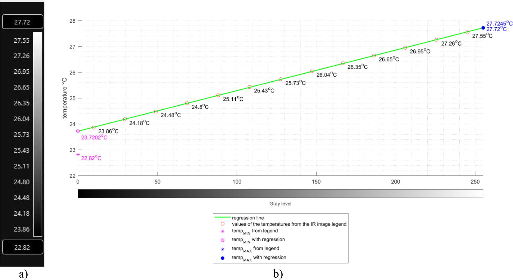
a. Legend of the infrared image; b. tempMin and tempMax directly from the IR image and with linear regression
(Source: Matlab simulation)
Figure no. 4 shows the temporal evolution of the minimum and maximum temperature values estimated using regression of the intermediate values from the IR image legend.
The temporal evolution of the minimum and maximum temperature values estimated using regression of the intermediate values from the IR image legend
(Source: Matlab simulation)
To convert the grayscale value of the pixel to a temperature value, a linear transformation g(x) = m · x + n was used, which is also graphically described in Figure no. 5.
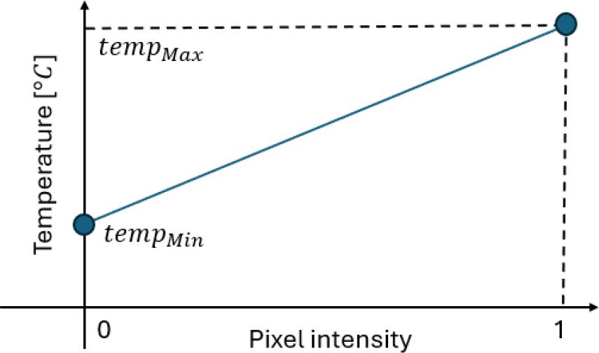
Graphical representation of the linear conversion from grayscale image to temperature
(Source: Matlab simulation)
Knowing the minimum and the maximum temperature, and the fact that these values are correlated with the darkest respectively the brightest pixel of the frame, the relation is captured in the following system of equations:
Solving for the slope and intercept, the resulting linear equation becomes:
Starting from equation above, each intensity of the pixel of coordinates (i, j) of the frame can be transformed in a temperature value using the linear transformation from equation 1:
- –
O(i, j, f) = the temperature of the pixel of coordinates (i, j) from frame f
- –
tempMin(f) = the minimum temperature of frame f
- –
tempMax(f) = the maximum temperature of frame f
- –
G(i, j, f) = the intensity of the pixel of coordinates (i, j)from frame f
The effect of equation (1) is that:
- –
the pixel with the intensity value equal to 0 will correspond to the minimum value of the temperature (tempMin) of frame f
- –
the pixel with the intensity value equal to 1 will correspond to the maximum value of the temperature (tempMax) of frame f
- –
all the others values of the pixels from the interval [0‥1] will be linearly distributed between the minimum and the maximum values of the current frame f
To analyze the performance of the conversion from grayscale value to temperature, a comparison with the temperatures returned by the thermal camera was done. The Mean Square Error (MSE) was computed for each frame f, using equation 2.
- –
f = the index of the frame, f ∈ [1, N], is the number of frames
- –
m, n = the number of rows respectively the number of the columns of the image
- –
O = the temperature obtained with equation 1
- –
R = the temperature returned by the sensor of the camera
As indicated in equation 2, the MSE is not normalized. The mean MSE for the entire video is computed as in equation 3:
As can be seen in Figure no. 6, using Method 1 (described in Chapter 3.1.a), there are several frames for which, at the same time, sudden variations occur in both the minimum temperature and MSE, which means that the real minimum temperature was not the one displayed in the bottom box of the legend of IR image.
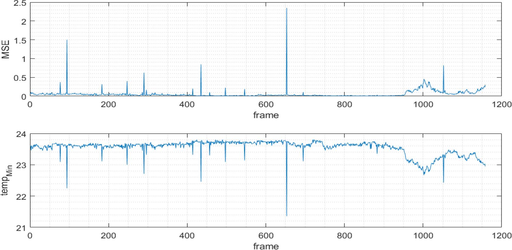
Top image: MSE for each frame; Bottom image: tempMin of each frame extracted from the bottom box of the legend of thermal image
(Source: Matlab simulation)
To correct these spikes, a median filter of length 3 was applied on the vector of the minimum temperatures extracted from the bottom box of the legend of thermal image. In this case, the spikes have been removed. But it is important to note that there still remains an interval around the frame with index 1000 for which the MSE remains high, interval marked with gray in Figure no. 7. These values are very closely related with the values of minimum temperatures which seem to have a strange decrease in that interval.
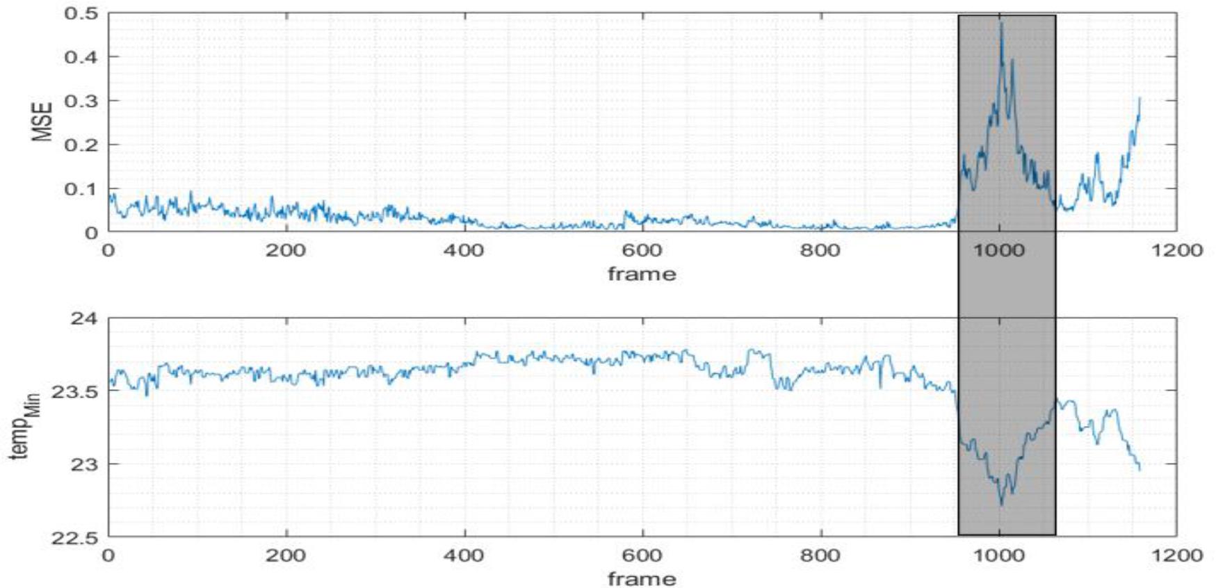
Top image: MSE for each frame; Bottom image: tempMin of each frame captured from the bottom box of the legend of thermal image, after median filtering
(Source: Matlab simulation)
Subsequently, Method 2 (described in Chapter 3.1.b) was applied to estimate the minimum and the maximum temperatures. A comparison between the extreme temperatures detected with Method 1 with median filter and Method 2 is presented in Figure no. 8, and their impact to MSE is shown in Figure no. 9.
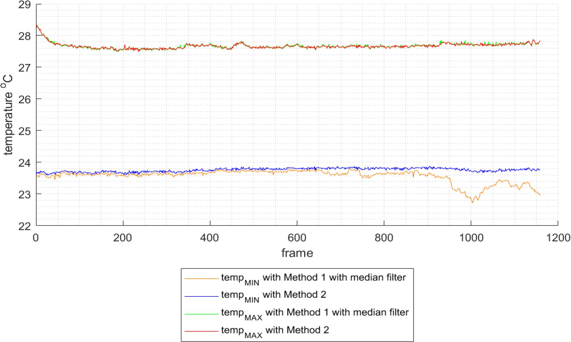
Minimum and maximum temperatures obtained with Method 1 with median filter and Method 2
(Source: Matlab simulation)
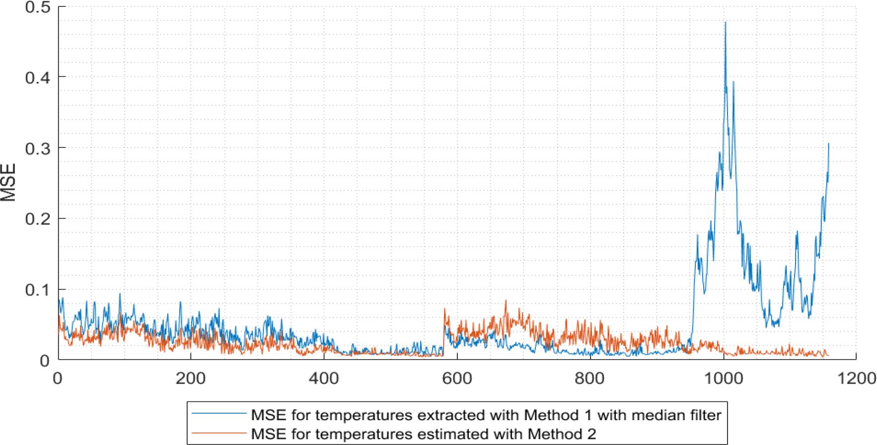
The evolution of MSE (not normalized)
(Source: Matlab simulation)
As can be noticed in Figure no. 8, the tempMax values are about the same, no matter the method used. But for the tempMin values, there are significantly differences around the frame with index 1000 where Method 2 seems to estimate more correctly the minimum temperature, which results from the Figure no. 9 where the values of MSE are visibly lower for Method 2.
Complementary to MSE, the R2 metric was also used, as it provides a relative measure of the model’s performance. The R2 metric was computed for each frame, using equation 4.
- –
f = the index of the frame, f ∈ [1, N], is the number of frames
- –
m, n = the number of rows respectively the number of the columns of the image
- –
O = the temperature obtained with equation 1
- –
R = the temperature returned by the sensor of the camera
- –
\bar R(f)
The mean for the entire video is computed with equation 5:
In Table no. 1 are the results of average MSE and R2 for the entire video, using the methods described before.
The mean values for MSE and R2
| Method to determine the tempMin and tempMax | MSEvideo | |
|---|---|---|
| Method 1 (ch. 3.1.a) without median filter | 0.0562 | 0.9668 |
| Method 1 (ch. 3.1.a) with median filter | 0.0490 | 0.9710 |
| Method 2 (ch. 3.1.b) | 0.0238 | 0.9861 |
As can be noticed, using Method 1 with median filter, an improvement of 12.81% for MSE for the entire video was obtained compared to Method 1 without median filter (from MSEvideo = 0.0562 to MSEvideo = 0.0490).
Using Method 2, an improvement of MSE with 57.65% was obtained compared to Method 1 without median filter and an improvement of 51.43% compared to Method 1 with median filter. Also, using Method 2, a value of closer to 1 was obtained, which means that the predicted values are very close to the actual values measured by the sensor of the camera.
The methods described achieve the conversion of pixel intensities into a map of temperatures and were tested on recorded frames with a FLIR infrared camera which provides the grayscale images with a legend of temperatures, but also a csv file with the real temperature values at each pixel position. The proposed method can be very useful for the analysis of the infrared images for which the temperatures recorded by the sensor are not stored or delivered to the user.
As shown by the results, it seems that the minimum and the maximum temperatures from the legend of infrared images are not on the regression line estimated using the intermediate points of the temperature legend. It was observed that placing the extreme points on the regression line, the average MSE for all the frames was improved with more than 50% and the R2 value is very close to 1.
Although linear regression is proven to be sufficient for the analyzed cases, the method itself could be extended to non-linear regressions (such as polynomial, logarithmic or exponential regression) for videos exhibiting more unusual temperature to grayscale relations.