
Table 1
List of datasets from Austria (AT), Switzerland (CH) and Italy (IT) naming sources, number of samples, land-use and mean, lowest (min) and highest (max) elevation of the sites sampled
Tabelle 1. listet die Datensammlungen aus Österreich (AT), Schweiz (CH) und Italien (IT) mit Quellen, Anzahl Bodenprobe, Landnutzung und mittlere (mean), minimale (min) und maximimale (max) Höhenlage der Probenstellen.
| Country | Made available by | number of samples | Land-use | elevation (m asl) | |||
|---|---|---|---|---|---|---|---|
| mean | min | max | |||||
| AT | our own dataset | 15 | Grassland | 909 | 672 | - | 1554 |
| AT | Upper Austria (BORIS) | 567 | cropland | 540 | 400 | - | 1140 |
| AT | Upper Austria (BORIS) | 656 | Grassland | 1047 | 410 | - | 2460 |
| AT | BAW (internal dataset) | 348 | Forest | 1024 | 400 | - | 2050 |
| AT | A. Bohner (other studies) | 18 | Grassland | 663 | 420 | - | 1830 |
| CH | J. Leifeld | 116 | Grassland | 760 | 430 | - | 1220 |
| IT | EURAC | 12 | Grassland | 1607 | 986 | - | 2043 |
[i] BORIS = official soil data base (https://www.umweltbundesamt.at/boris); BAW = Bundesanstalt für Wasserwirtschaft, Petzenkirchen; EURAC = Institute of Alpine Environment, Bolzano
Table 2
Mean, minimum (min) and maximum (max) values of soil depth, organic carbon (SOC), sand, silt, clay and bulk density according to the datasets: all data, cropland, forest and grassland (n = number of samples)
Tabelle 2. Mittlere (mean), minimale (min) und maximale (max) Werte der Bodenprobeentnahme, organischem Bodenkohlenstoff (SOC), Sand-, Schuff-, Tongehalten und der Bodenlagerungsdichten (BD) von ‚allen Daten‘, Ackerböden, Wald- und Grünlandböden (n = Anzahl Proben)
| parameter | all data (n = 1732) | cropland (n = 567) | forest (n = 348) | grassland (n = 817) | ||||||||||||
|---|---|---|---|---|---|---|---|---|---|---|---|---|---|---|---|---|
| mean | min | max | mean | min | max | mean | min | Max | mean | min | max | |||||
| Depth [cm] | 20 | 1 | - | 70 | 26 | 10 | - | 50 | 27 | 8 | - | 60 | 12 | 1 | - | 70 |
| SOC [mg g−1] | 39 | 1 | - | 295 | 19 | 4 | - | 120 | 32 | 10 | - | 185 | 55 | 1 | - | 295 |
| Sand [mg g−1] | 280 | 0 | - | 910 | 217 | 0 | - | 721 | 35 | 21 | - | 717 | 289 | 18 | - | 910 |
| Silt [mg g−1] | 538 | 2 | - | 934 | 587 | 172 | - | 934 | 446 | 172 | - | 703 | 544 | 20 | - | 882 |
| Clay [mg g−1] | 184 | 1 | - | 701 | 197 | 35 | - | 467 | 207 | 36 | - | 701 | 167 | 10 | - | 560 |
| BD [g cm−3] | 1.2 | 0.3 | - | 2.2 | 1.4 | 0.5 | - | 1.7 | 1 | 0.4 | - | 2.2 | 1.1 | 0.3 | - | 1.7 |
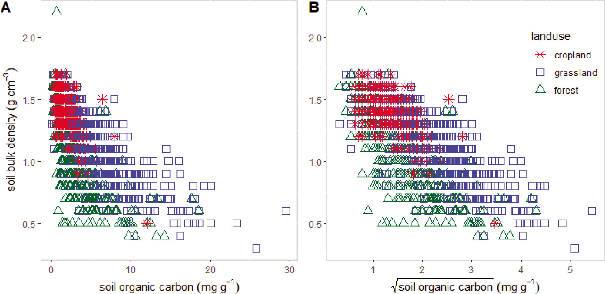
Figure 1
Measured soil bulk densities from cropland (star), forest (triangle) and grassland (squares) soils versus A) soil organic content and B) squared root of soil organic carbon
Abbildung 1. gemessene Bodenlagerungsdichten von Acker- (Sterne), Wald- (Triangel) und Grünlandböden (Quadrate) versus A) gemessenen organischen Bodenkohlenstoff und B) Wurzel des organischen Bodenkohlenstoffs
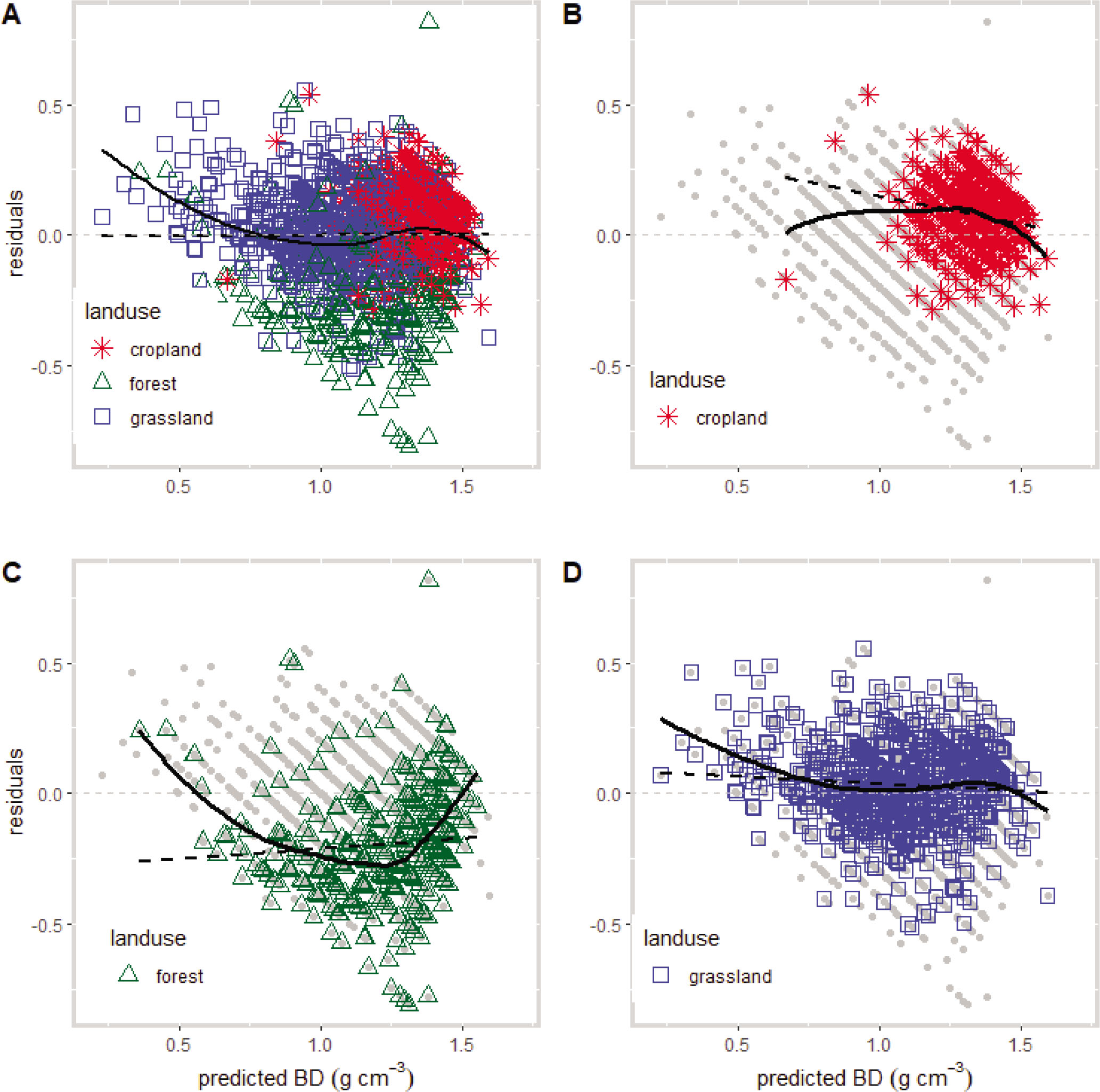
Figure 2
Residuals versus predicted soil bulk densities (BD) with regression line (dashed) and lowest smoothing line (solid) of A) all data, B) cropland, C) forest and D) grassland sites.
Abbildung 2. Die Residuen versus modellierten Bodenlagerungsdichten (BD) mit der lineare Regressionsline (gestrichelt) und LOWESS-Spline-Linie (durchgezogen) von A) ‚alle Daten‘, B) Ackerböden, C) Wald- und D) Grünlandböden.
Table 3
Coefficients of the linear model equations (EQ) and the evaluation of the models by R squared (R2), root mean squared error (RMSE) and percentage of uncertainty (PU) together with the validation by the mean squared R (mR2) of the cross validation (CV)
Tabelle 3. Die Koeffizienten der linearen Gleichungen (EQ) und die Evaluierung der Modelle anhand des Bestimmtheitsmaß (R2), Wurzel der Mittlere quadratische Abweichung (RMSE) und dem Prozent der Unsicherheit (PU) gemeinsam mit dem Ergebnis der Validierung durch mittleres Bestimmtheitsmaß (mR2) aus der Kreuzvalidierung (CV)
| EQ | landuse | Intercept | Depth [cm] | SOC−0.5 [%]0.5 | Silt [%] | Clay [%] | R2 | RMSE | PU [%] | CV mR2 |
|---|---|---|---|---|---|---|---|---|---|---|
| 1 | all data | 1.650 | −0.0022*** | −0.3157*** | 0.0028* | 0.58 | 0.190 | 21 | 0.57 | |
| 2 | cropland | 1.873 | −0.0021*** | −0.3042*** | 0.43 | 0,105 | 9 | 0.41 | ||
| 3 | forest | 1.523 | −0.3199*** | 0.58 | 0.205 | 25 | 0.56 | |||
| 4 | grassland | 1.698 | −0.2737*** | 0.0009** | −0.0020** | 0.65 | 0.171 | 17 | 0.65 | |
| 5 | all data | 1.682 | −0.2738*** | 0.55 | 0.197 | 24 | ||||
| 6 | cropland | 1.720 | −0.2306*** | 0.41 | 0.107 | 9 | ||||
| 7 | grassland | 1.693 | −0.2635*** | 0.65 | 0.157 | 18 |
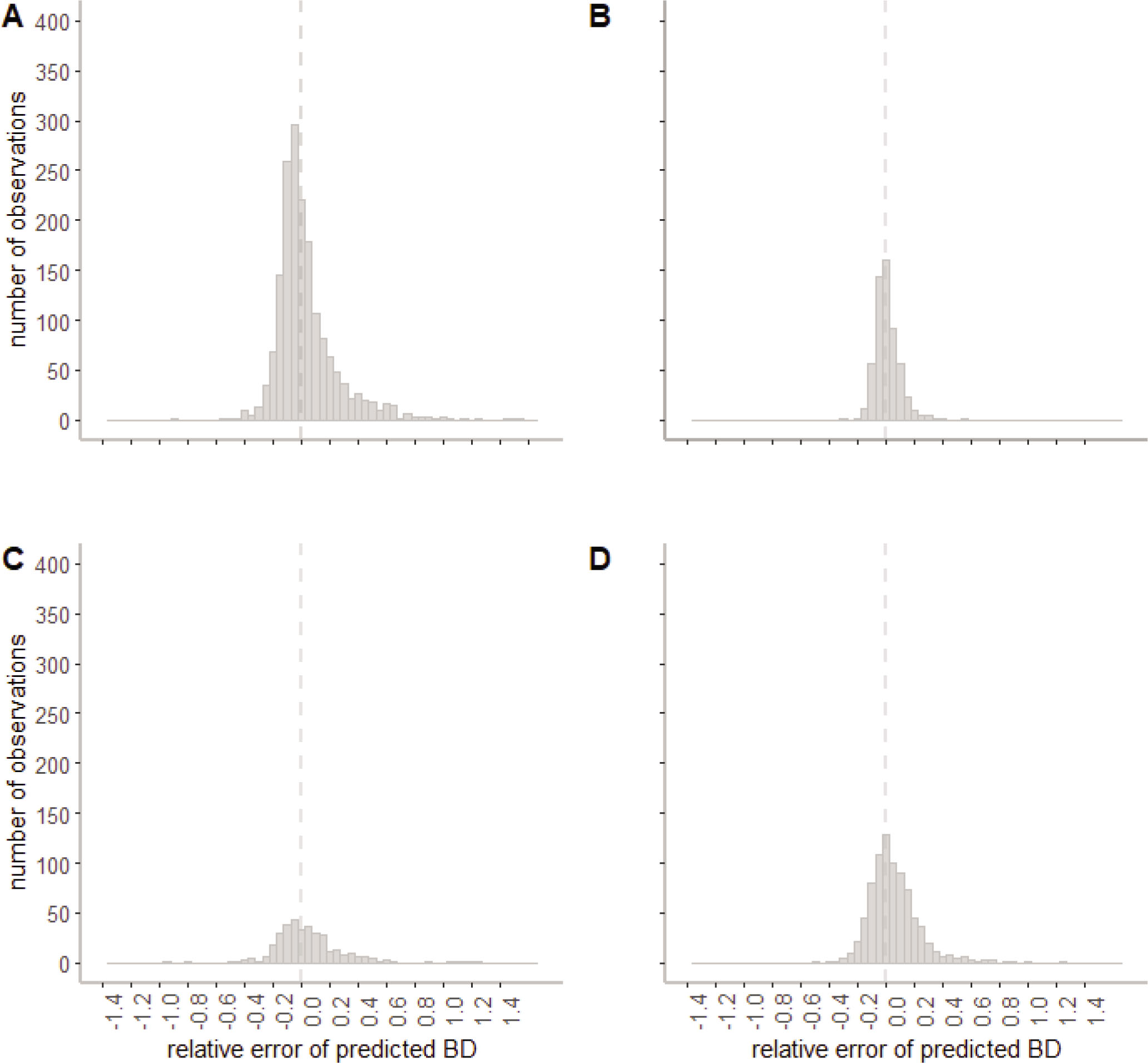
Figure 3
Histograms showing the bias (relative error) of predicted soil bulk density (BD) of A) all data, B) cropland C) forest and D) grassland respectively Abbildung 3. Histogramm mit der Verzerrung (relative Fehler) der geschätzten Bodenlagerungsdichten (BD) bei A) ‚alle Daten‘, B) Ackerböden, C) Wald- und D) Grünlandböden
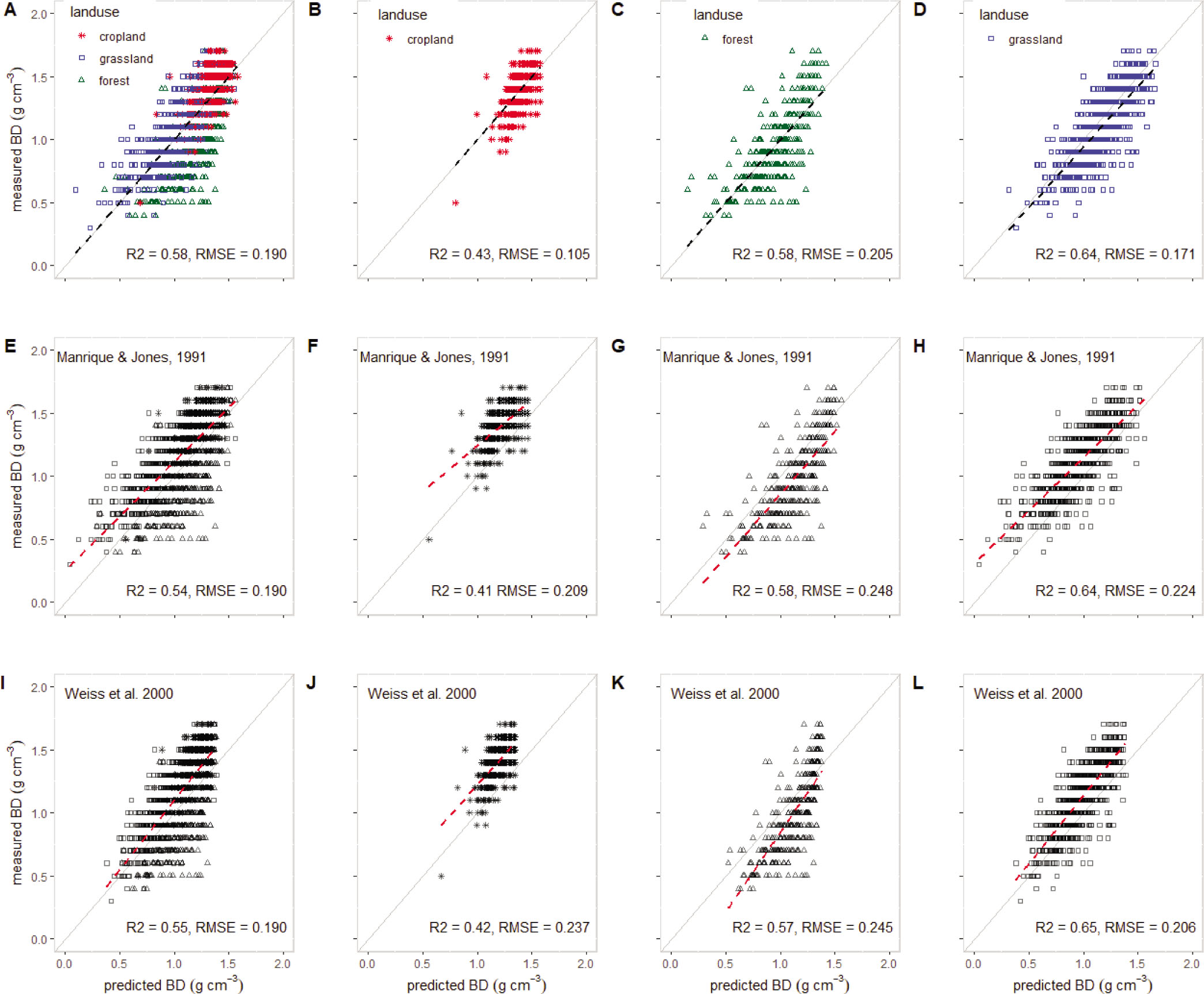
Figure 4
Performance of measured versus predicted soil bulk density (BD) including regression line (dashed) for “all data”, “cropland”, “forest” and “grassland” datasets applying A – D the best of regional equations from this study, E – H the model of Manrique and Jones (1991) and I – L the model used by Weiss et al (2000). R2 and RMSE describe the goodness of the functions
Abbildung 4. Modellierte versus gemessene Bodenlagerungsdichten mit Regressionsline (gestrichelt) für alle Datensets (‚all data‘, ‚cropland‘, ‚forest‘ und ‚grassland‘) in A – D anhand der regional kalibrierten Gleichungen dieser Studie, E – H berechnet mit dem Modell von Manruiqe und Jones (1991) und I – L das Modell verwendet von Weiss et al. (2000). R2 und RMSE geben die Güte der Gleichungen wieder.