
Table 1
Indicators to be evaluated for the ecological assessment of fluvial areas. In the present table, the indicators are divided in automatically assessable or not.
Tabelle 1. Indikatoren zur Evaluation der ökologischen Bewertung von Flusslandschaften. Die Indikatoren sind unterteilt in automatisch bewertbar oder nicht automatisch bewertbar.
| Indicators assessable through semi-automatic data processing | Indicators differently assessable |
|---|---|
| Land use | Vertical continuity |
| Lateral continuity | Hydrologic regime |
| Longitudinal continuity | Chemical quality |
| Morphological heterogeneity | Macrobenthos community |
| Retention capability | Carbon footprint |
| Fish suitability | |
| Riparian zone vegetation | |
| Riparian zone width | |
| Riparian zone continuity | |
| Carbon sequestration |
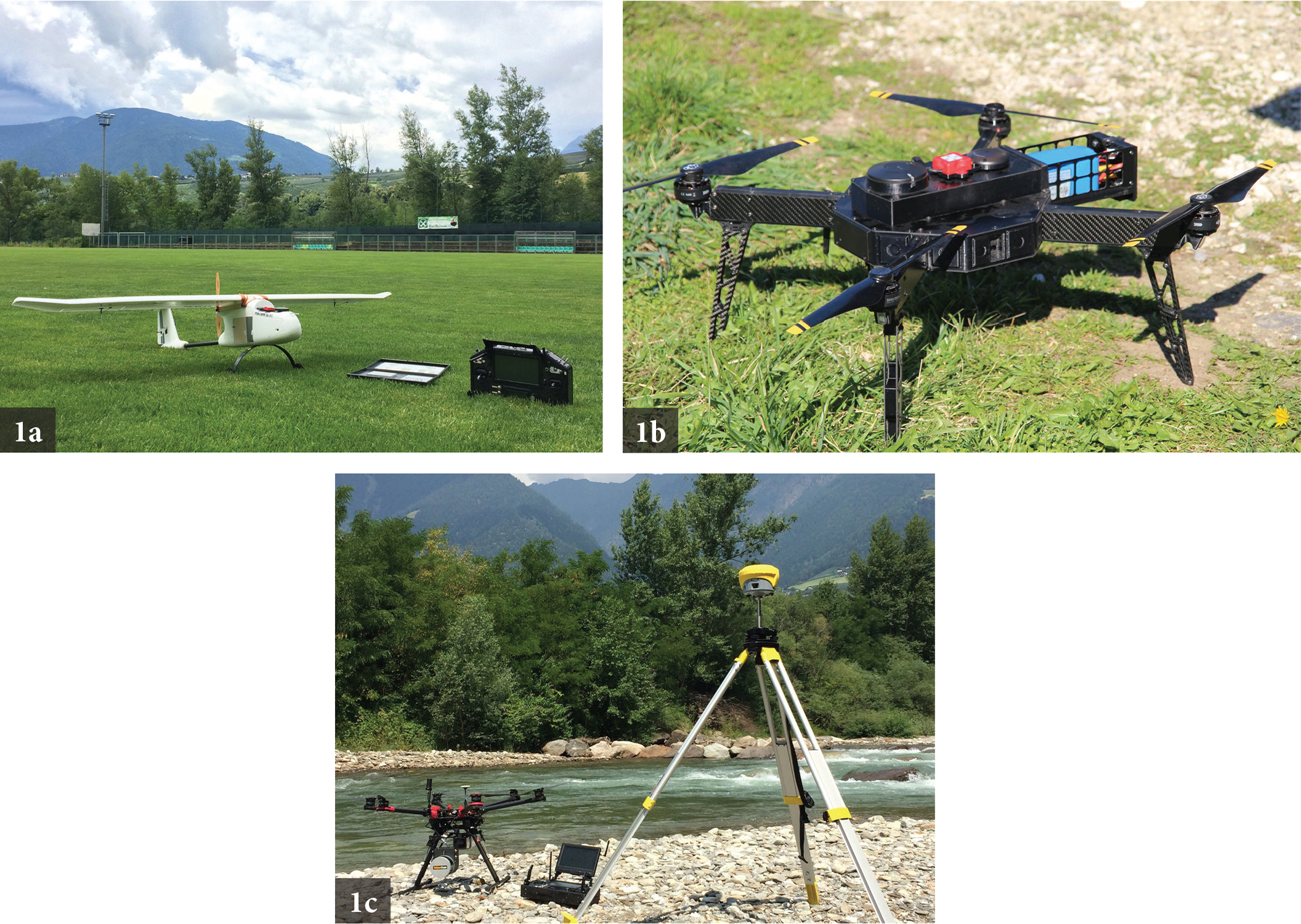
Figure 1
The three aircrafts used for the monitoring purposes: (a) AGRI-1900, (b) Q4E, (c) DJI S900 with the RTK-GNSS base for RINEX files collection. The first two solutions are two prototypes specifically developed to answer to the project’s requirement, while the third is a commercial UAV, which has been modified to carry the Yellowscan Surveyor sensor.
Abbildung 1. Die drei zu Überwachungszwecken verwendeten Flugobjekte: (a) AGRI-1900, (b) Q4E, (c) DJI S900 mit der RTK-GNSS-Basis für die Sammlung von RINEX-Daten. Die ersten beiden UAV sind Prototypen, die speziell für die Anforderungen des Projekts entwickelt wurden. Das dritte ist ein kommerzielles Flugobjekt, das für den Yellowscan Surveyor-Sensor modifiziert wurde.
Table 2
Summary of the main features of the rotary-wing UAVs used for the environmental surveys.
Tabelle 2. Zusammenfassung der Hauptmerkmale der Drehflügel-UAVs, die für die Umweltuntersuchungen verwendet werden.
| Mavtech Q4E | Mavtech DJI S900 | |
|---|---|---|
| Number of rotors (−) | 4 | 6 |
| Weight (kg) | 3.5 | 8.2 |
| Diagonal wheelbase (m) | 0.59 | 0.9 |
| Endurance (min) | 20–25 | 15 |
| Cruise speed (m/s) | 6 | 3 |
| Maximum area coverable (ha) | 4 | 5 |
| Equipment installable on-board | SONY RX-100 | Yellowscan surveyor |
| Micasense RedEdge-M |
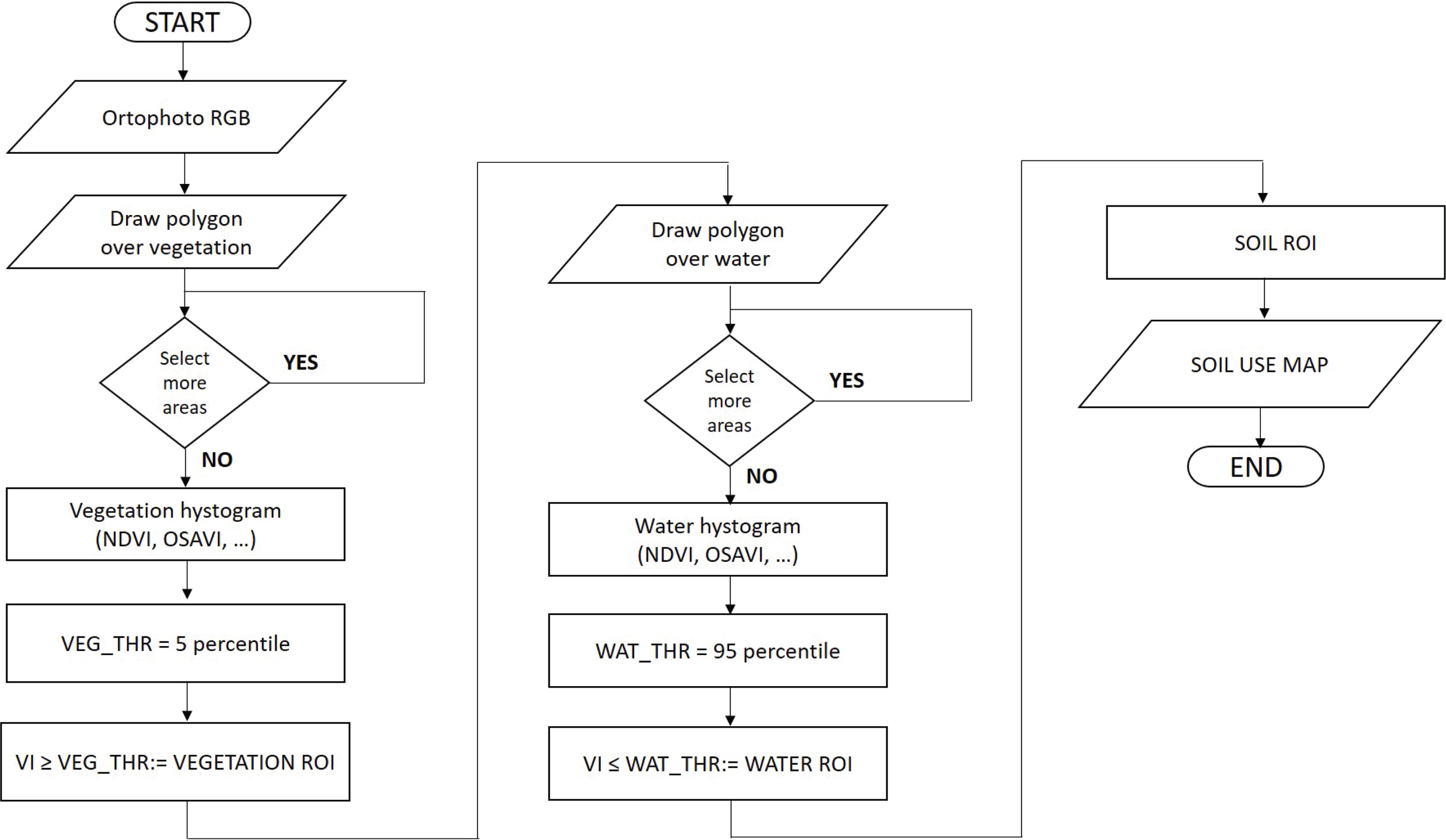
Figure 2
Land use algorithm flow-chart.
Abbildung 2. Flow-Chart des Bodennutzungsalgorithmuses.
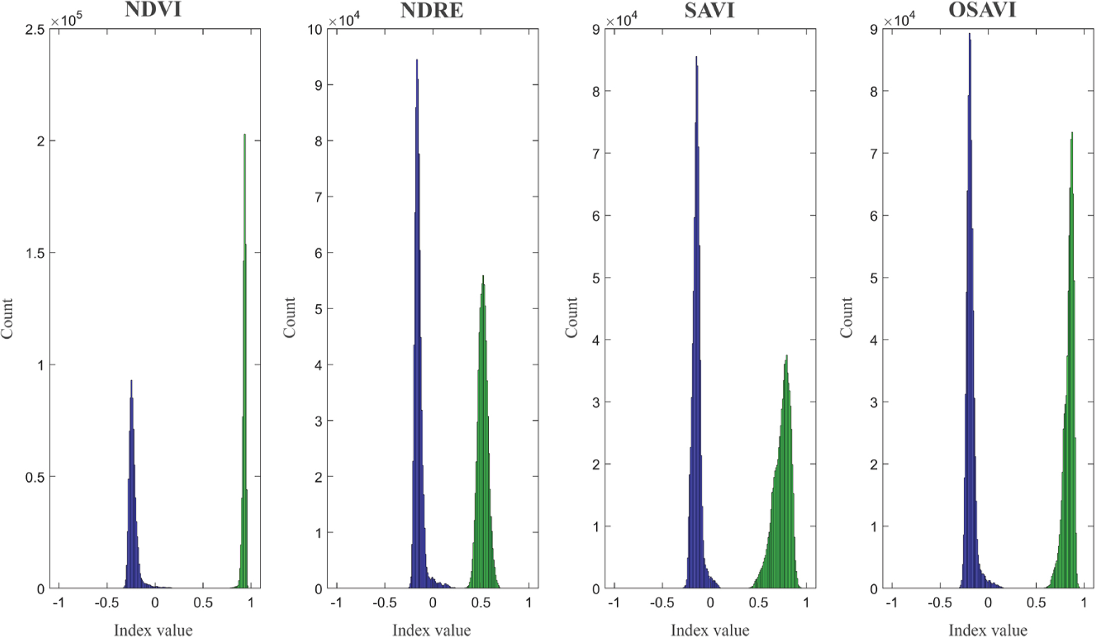
Figure 3
Histogram of the statistical distribution of the Vegetative Indexes for the selected area covered by vegetation (green histogram) and water (blue histogram). To distinguish between vegetation and water bodies, the procedure will select the most useful vegetative index, which has the biggest difference between the two distributions. In this way, a clear classification is expected.
Abbildung 3. Histogramm der statistischen Verteilung der Vegetativen Indizes für das ausgewählte Gebiet, das von Vegetation (grünes Histogramm) und Wasser (blaues Histogramm) bedeckt ist. Um zwischen Vegetation und Gewässern zu unterscheiden, wird jener Vegetationsindex ausgewählt, der den größten Unterschied zwischen den beiden Verteilungen aufweist. Auf diese Weise wird eine eindeutige Zuordnung erwartet.
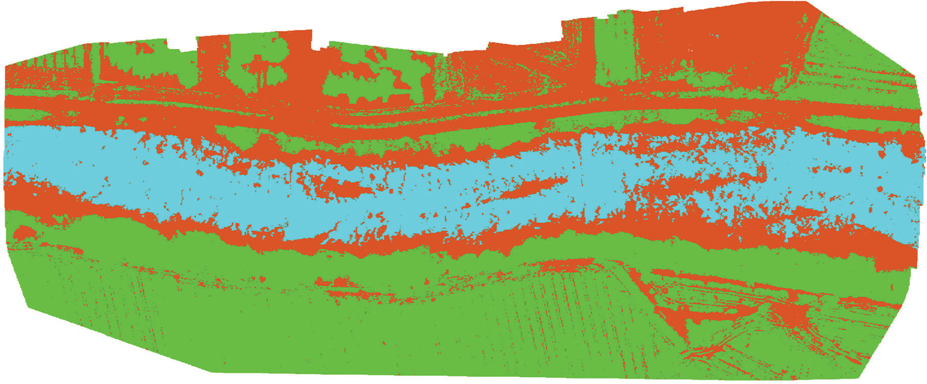
Figure 4
Land use thematic map of the Adige river, where green represents vegetation, brown soil and light blue water.
Abbildung 4. Thematische Landnutzungskarte der Etsch, wobei grün für Vegetation, braun für Boden und hellblau für Wasser steht.
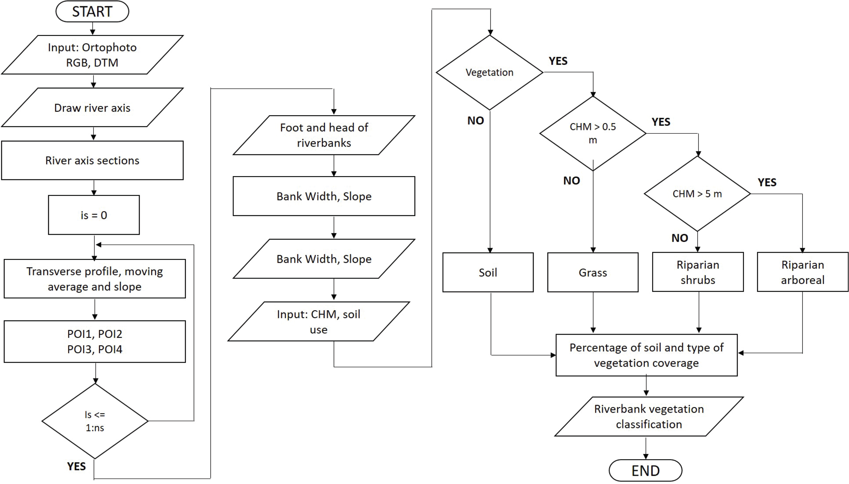
Figure 5
Flow-chart of the algorithm for riverbanks identification and the classification of the riparian strip vegetation.
Abbildung 5. Flow-Chart des Algorithmus zur Identifizierung des Ufers und der Klassifizierung des Bodens und der Ufervegetation.
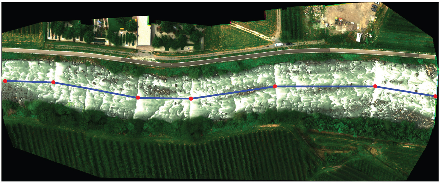
Figure 6
Example of river’s axle drawing (blue line). Red dots correspond to the building points selected to draw a line segment. In this example, the river’s flow is from left to right.
Abbildung 6. Beispiel der Zeichnung der Flussachse (blaue Linie). Rote Punkte entsprechen den Punkten, die zum Zeichnen eines Liniensegments ausgewählt wurden. In diesem Beispiel fließt der Fluss von links nach rechts.
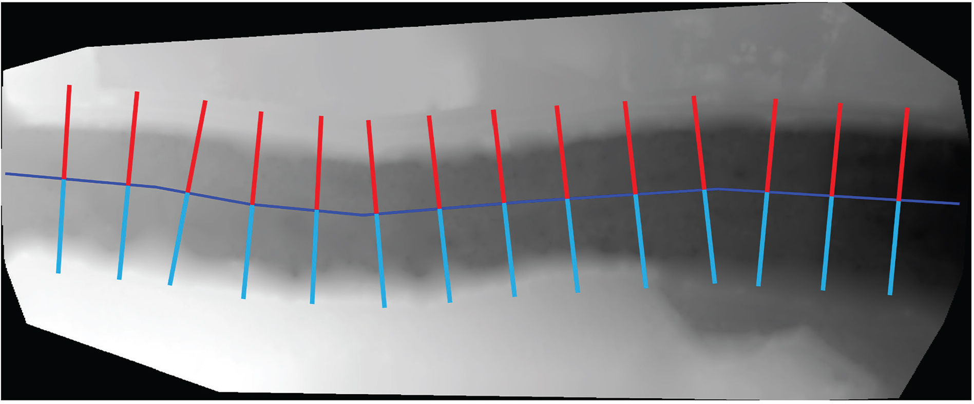
Figure 7
Automatic definition of the river’s transverse sections using the middle line of the river (dark blue line). The transverse sections are colored in red or light blue line depending on the side of the bank (right or left).
Abbildung 7. Automatische Definition der Flussquerschnitte anhand der Mittellinie des Flusses (dunkelblaue Linie). Die Querschnitte sind je nach Uferseite (rechts oder links) rot oder hellblau eingefärbt.
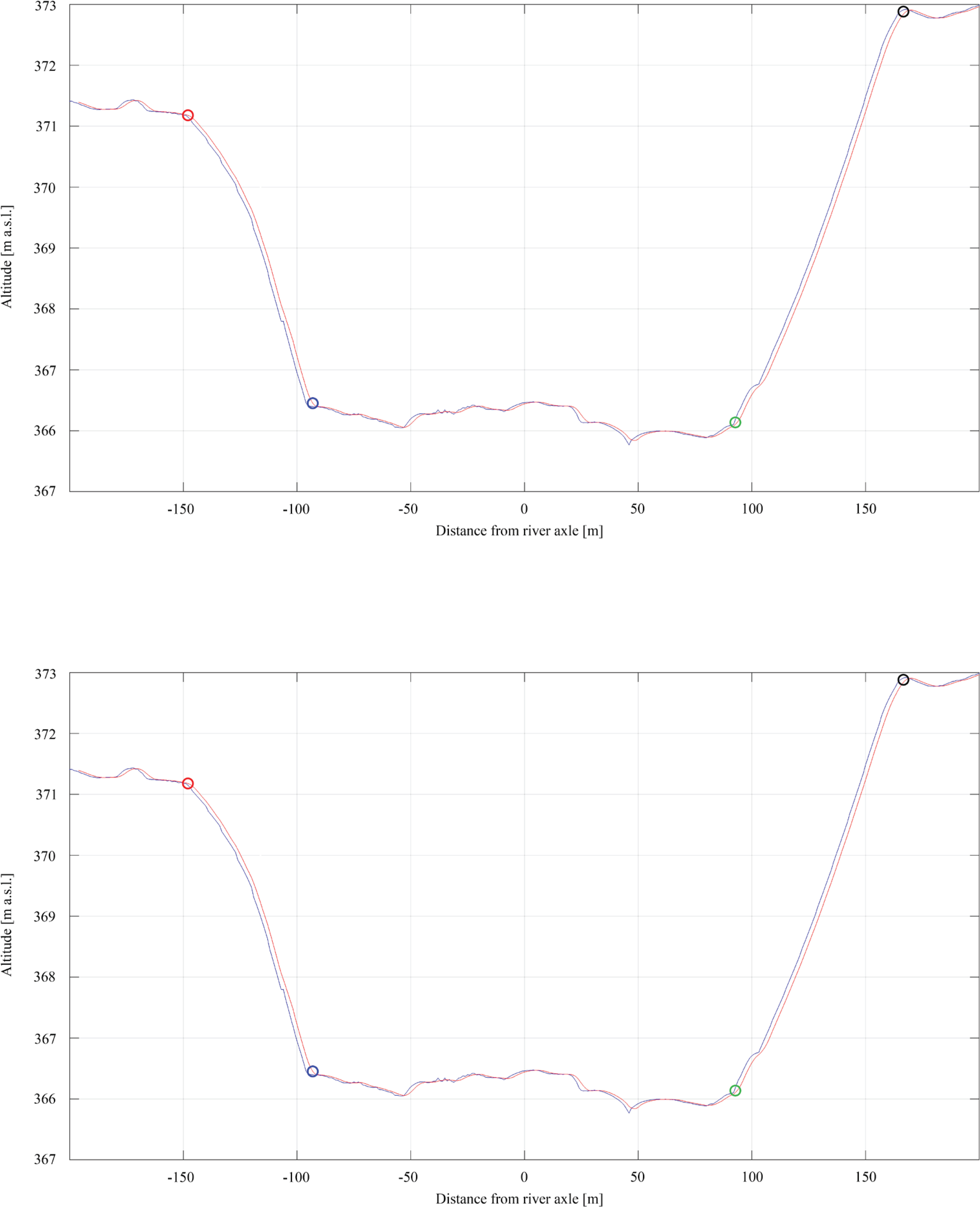
Figure 8
Procedure for the identification of the bottom and top of both riversides and the terrain profile for each transversal section previously identified. In a), the blue line represents the first derivative (slope) of the section, while the red one represents the moving average of the calculated first derivative. The black dashed line represents the thresholds used to detect the POIs: when the moving average of the derivate overpasses these thresholds, the POIs are set-up, identifying the top (POI1) and bottom (POI2) of the left riverside (red and blue circle) and the bottom (POI3) and top (POI4) of the right riverside (green and black circle). In b), the riverside terrain profile is reported. The blue line represents the actual height of the section, while the red line represents the moving average of the height of the section. Also, the four POIs are reported in this figure.
Abbildung 8. Verfahren zur Identifizierung der Unter- und Oberseite beider Flussufer und des Geländes für jeden zuvor identifizierten Querschnitt. In a) repräsentiert die blaue Linie die erste Ableitung (Steigung) des Abschnitts, während die rote den gleitenden Durchschnitt der berechneten ersten Ableitung darstellt. Die schwarze gestrichelte Linie stellt die Schwellwerte dar, die zum Ermitteln der POIs verwendet werden: Wenn der gleitende Durchschnitt der Ableitung diese Schwellwerte überschreitet, werden die POIs eingerichtet, die den oberen (POI1) und unteren (POI2) Bereich des linken Flussufers (roter und blauer Kreis) sowie die Unterseite (POI3) und die Oberseite (POI4) des rechten Flussufers (grüner und schwarzer Kreis) identifizieren. In b) wird das Profil des Flussgeländes dargestellt. Die blaue Linie stellt die tatsächliche Höhe des Abschnitts dar, während die rote Linie den gleitenden Durchschnitt der Höhe des Abschnitts abbildet. In dieser Abbildung sind auch die vier POIs eingezeichnet.
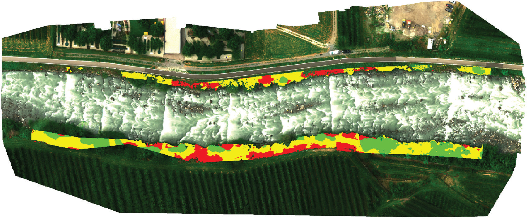
Figure 9
Classification layer overlapping an RGB image in the study area. Graphical result of algorithm procedures for riverbanks, riparian and alluvial riparian vegetation (the red, yellow and green colors refer to the herbaceous layer, riparian shrubs and riparian arboreal, respectively).
Abbildung 9. Klassifizierungsebene, die ein RGB-Bild im Untersuchungsgebiet überlappt. Grafisches Ergebnis der Algorithmen für Flussufer, Auen- und Ufervegetation (die Farben Rot, Gelb und Grün beziehen sich auf die krautige Schicht, die Auensträucher bzw. auf die Auenbäume).
Table 3
Area in percentage obtained through the validation of the automatic analysis procedure.
Tabelle 3. Fläche in Prozent, die durch die Validierung des automatischen Analyseverfahrens erhalten wurde.
| Visual survey Area (%) | Automatic survey Area (%) | Differences Area (%) | |
|---|---|---|---|
| Vegetation | 53.2 | 50.3 | −2.9 |
| Water | 27.2 | 21.0 | −6.2 |
| Ground | 19.6 | 28.7 | 9.1 |