
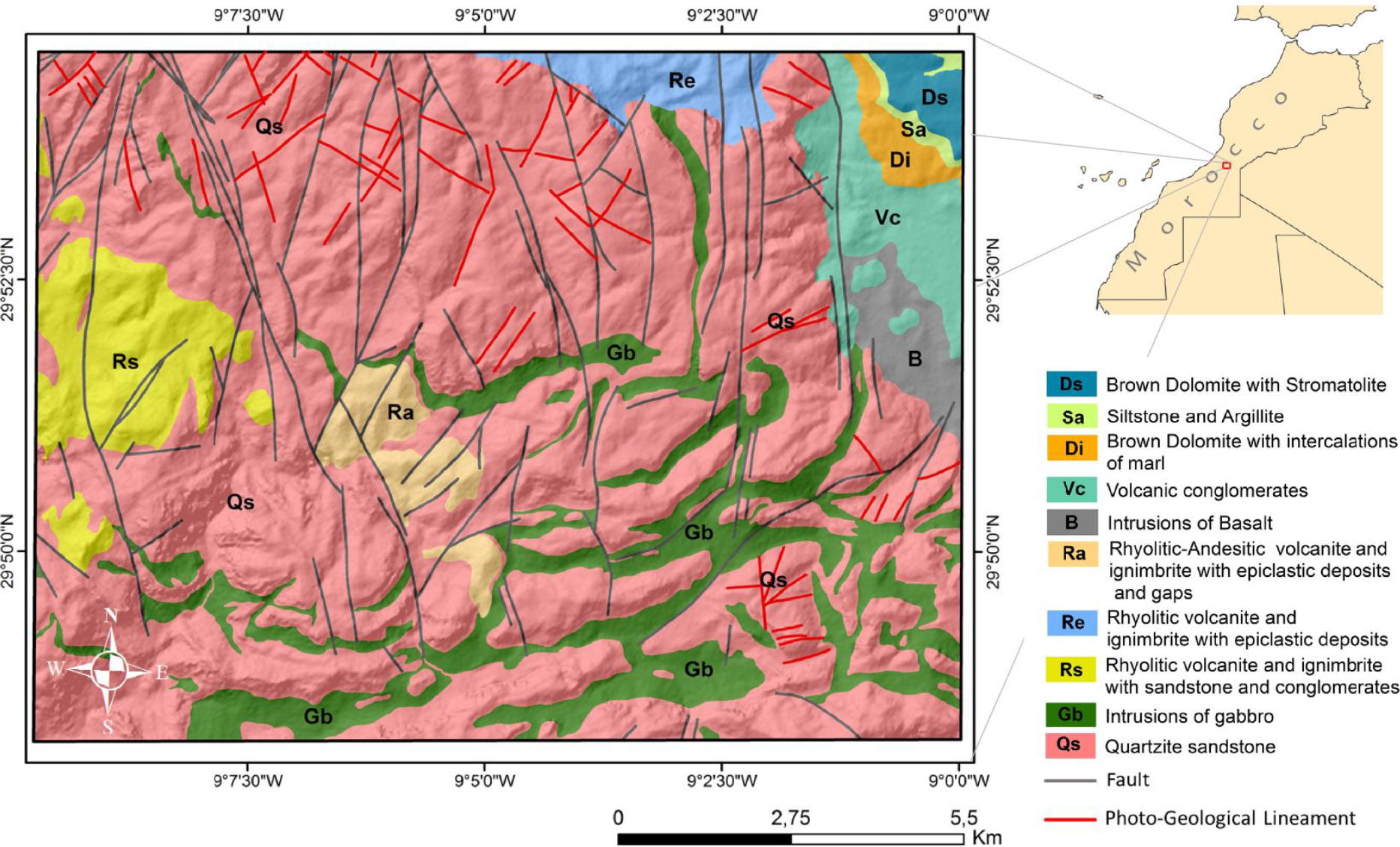
Figure 1.
Lithological map of the study area (modified from the Tanalt geological map)
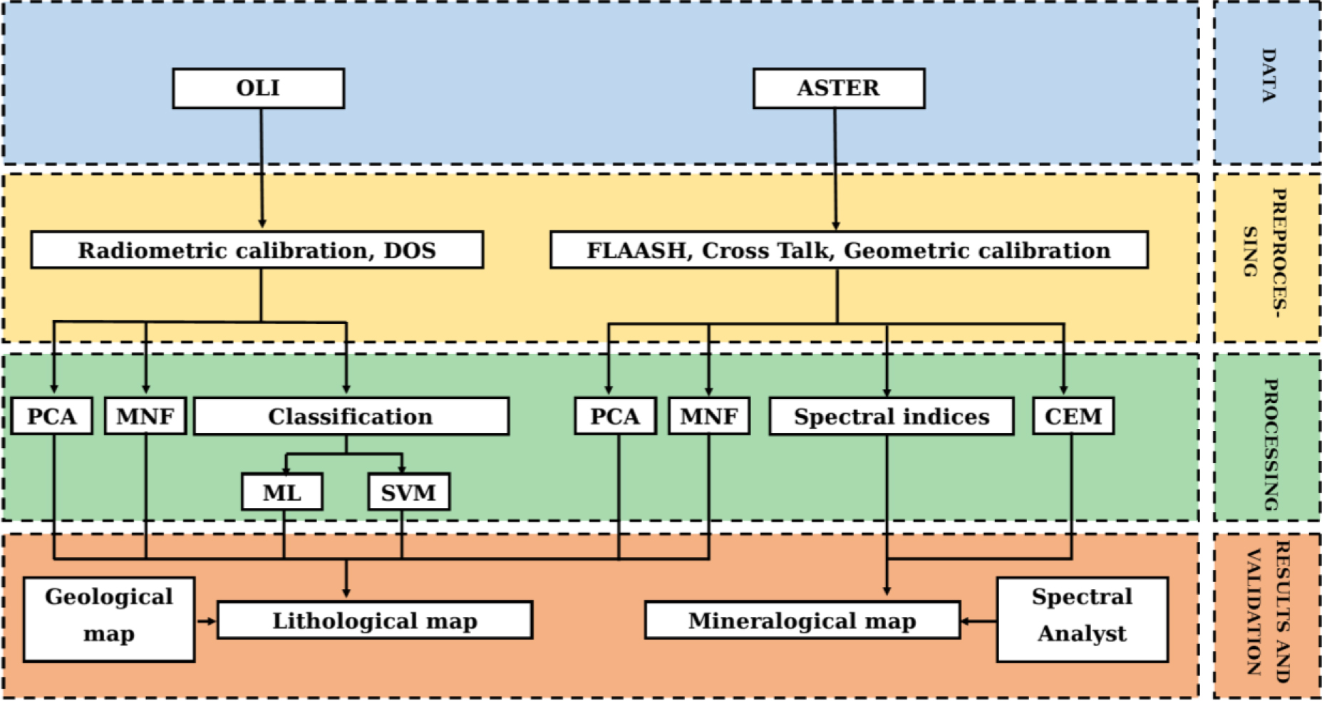
Figure 2.
The methodology flowchart
Table 1.
Terra ASTER data characteristics
| Bands | Covered Spectrum | Wavelengths (μm) | Resolution (m) |
|---|---|---|---|
| 1 | VNIR | 0.520–0.600 | 15 |
| 2 | VNIR | 0.630–0.690 | 15 |
| 3N | VNIR | 0.760–0.860 | 15 |
| 3B | VNIR | 0.760–0.860 | 15 |
| 4 | SWIR | 1.600–1.700 | 30 |
| 5 | SWIR | 2.145–2.185 | 30 |
| 6 | SWIR | 2.185–2.225 | 30 |
| 7 | SWIR | 2.235–2.285 | 30 |
| 8 | SWIR | 2.295–2.365 | 30 |
| 9 | SWIR | 2.365–2.430 | 30 |
| 10 | TIR | 8.125–8.475 | 90 |
| 11 | TIR | 8.475–8.825 | 90 |
| 12 | TIR | 8.925–9.275 | 90 |
| 13 | TIR | 10.25–10.95 | 90 |
| 14 | TIR | 10.95–11.65 | 90 |
Table 2.
Landsat-8 OLI data characteristics
| Bands | Wavelengths (μm) | Spatial resolution (m) |
|---|---|---|
| Band 1-coastal/aerosol | 0.43–0.45 | 30 |
| Band 2-Blue | 0.45–0.51 | 30 |
| Band 3-Green | 0.53–0.59 | 30 |
| Band 4-Red | 0.64–0.67 | 15 |
| Band 5-NIR | 0.85–0.88 | 30 |
| Band 6-SWIR 1 | 1.57–1.65 | 30 |
| Band 7-SWIR 2 | 2.11–2.29 | 30 |
| Band 8-Panchromatic | 0.50–0.68 | 15 |
| Band 9-Cirrus | 1.36–1.38 | 30 |
Table 3.
PCA eigenvector matrix of ASTER bands
| Eigenvectors | Eigenvalues (%) | Band 1 | Band 2 | Band 3 | Band 4 | Band 5 | Band 6 | Band 7 | Band 8 | Band 9 |
|---|---|---|---|---|---|---|---|---|---|---|
| PC 1 | 83.49 | -0.2073 | -0.3643 | -0.3000 | -0.4017 | -0.3157 | -0.3159 | -0.3434 | -0.3354 | -0.3779 |
| PC 2 | 8.61 | 0.3157 | 0.3620 | 0.6760 | 0.0359 | -0.1632 | -0.2192 | -0.2168 | -0.2680 | -0.3425 |
| PC 3 | 3.95 | -0.3816 | -0.5550 | 0.3412 | 0.5935 | 0.1125 | 0.0629 | 0.0189 | -0.1203 | -0.2144 |
| PC 4 | 2.31 | 0.2198 | 0.2946 | -0.5600 | 0.5047 | 0.1437 | -0.0375 | 0.0426 | -0.1342 | -0.5046 |
| PC 5 | 0.54 | 0.2128 | -0.1446 | 0.0484 | -0.2907 | 0.2730 | 0.7915 | -0.1968 | -0.1344 | -0.2983 |
| PC 6 | 0.4 | 0.1262 | -0.2003 | 0.1268 | -0.2920 | 0.1665 | -0.2261 | 0.5204 | 0.4782 | -0.5139 |
| PC 7 | 0.34 | -0.7725 | 0.5273 | 0.0629 | -0.1636 | 0.0905 | 0.1434 | 0.1037 | -0.0191 | -0.2333 |
| PC 8 | 0.20 | 0.0066 | -0.0244 | 0.0206 | -0.1657 | 0.8205 | -0.3631 | -0.0296 | -0.3749 | 0.1572 |
| PC 9 | 0.15 | -0.0722 | 0.0395 | 0.0020 | 0.0785 | 0.2378 | -0.1289 | -0.7152 | 0.6287 | -0.0825 |
Table 4.
PCA eigenvector matrix of OLI bands
| Eigenvectors | Eigenvalues (%) | Band 1 | Band 2 | Band 3 | Band 4 | Band 5 | Band 6 | Band 7 |
|---|---|---|---|---|---|---|---|---|
| PC 1 | 94.505 | -0.09192 | -0.12474 | -0.2078 | -0.33462 | -0.48452 | -0.60072 | -0.47457 |
| PC 2 | 3.398 | 0.000397 | -0.00519 | 0.024592 | -0.13446 | 0.842454 | -0.25154 | -0.45639 |
| PC 3 | 1.620 | 0.222355 | 0.292138 | 0.389118 | 0.690656 | -0.08932 | -0.46946 | -0.09177 |
| PC 4 | 0.279 | -0.12715 | -0.17061 | -0.22221 | -0.03729 | 0.213198 | -0.58625 | 0.717502 |
| PC 5 | 0.176 | 0.519782 | 0.523961 | 0.26547 | -0.58028 | -0.01976 | -0.096 | 0.196193 |
| PC 6 | 0.018 | -0.44877 | -0.26373 | 0.815732 | -0.2339 | -0.04026 | -0.05046 | 0.068967 |
| PC 7 | 0.003 | -0.67407 | 0.72517 | -0.13975 | -0.01132 | 0.00846 | -0.00293 | 0.004203 |
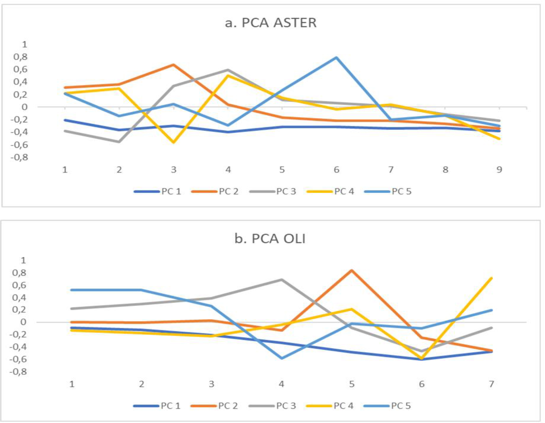
Figure 3.
Eigenvector loading trend graphical representation extracted from the first five (a) ASTER and (b) OLI PC bands from data in Tables 3 and 4
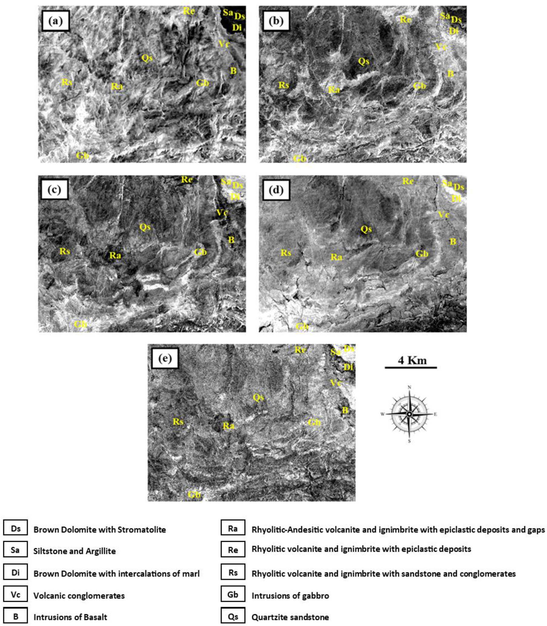
Figure 4.
PC images of ASTER: (a) PC1; (b) PC2; (c) PC3; (d) PC4; (e) PC7
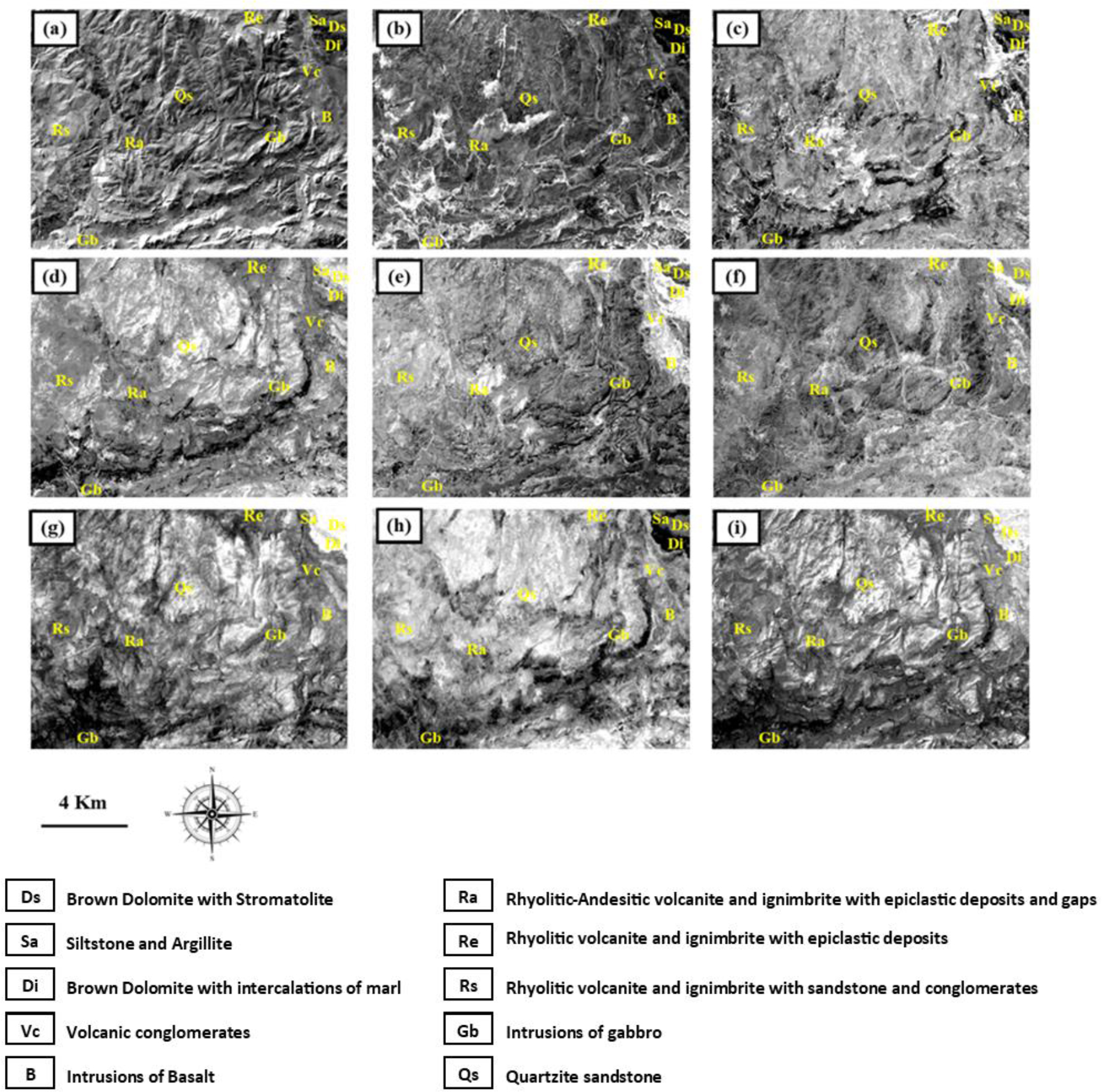
Figure 5.
PCA and MNF extracted images of: (a) OLI PC1; (b) OLI PC2; (c) OLI PC3; (d) OLI PC4; (e) OLI PC5; (f) OLI PC6; (g) ASTER MNF 1; (h) ASTER MNF 2; (i) OLI MNF1
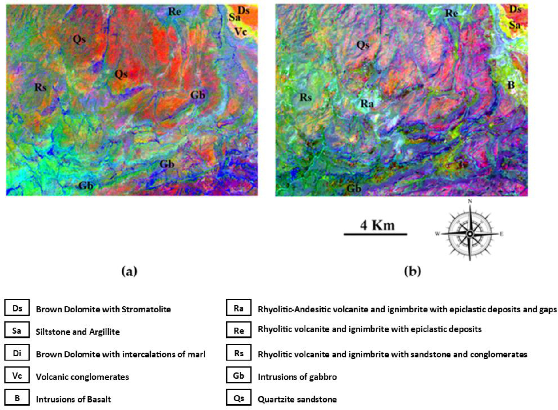
Figure 6.
(a) FCC ASTER MNF1, PC4, and PC2; (b) FCC OLI MNF1, PC5 and PC3
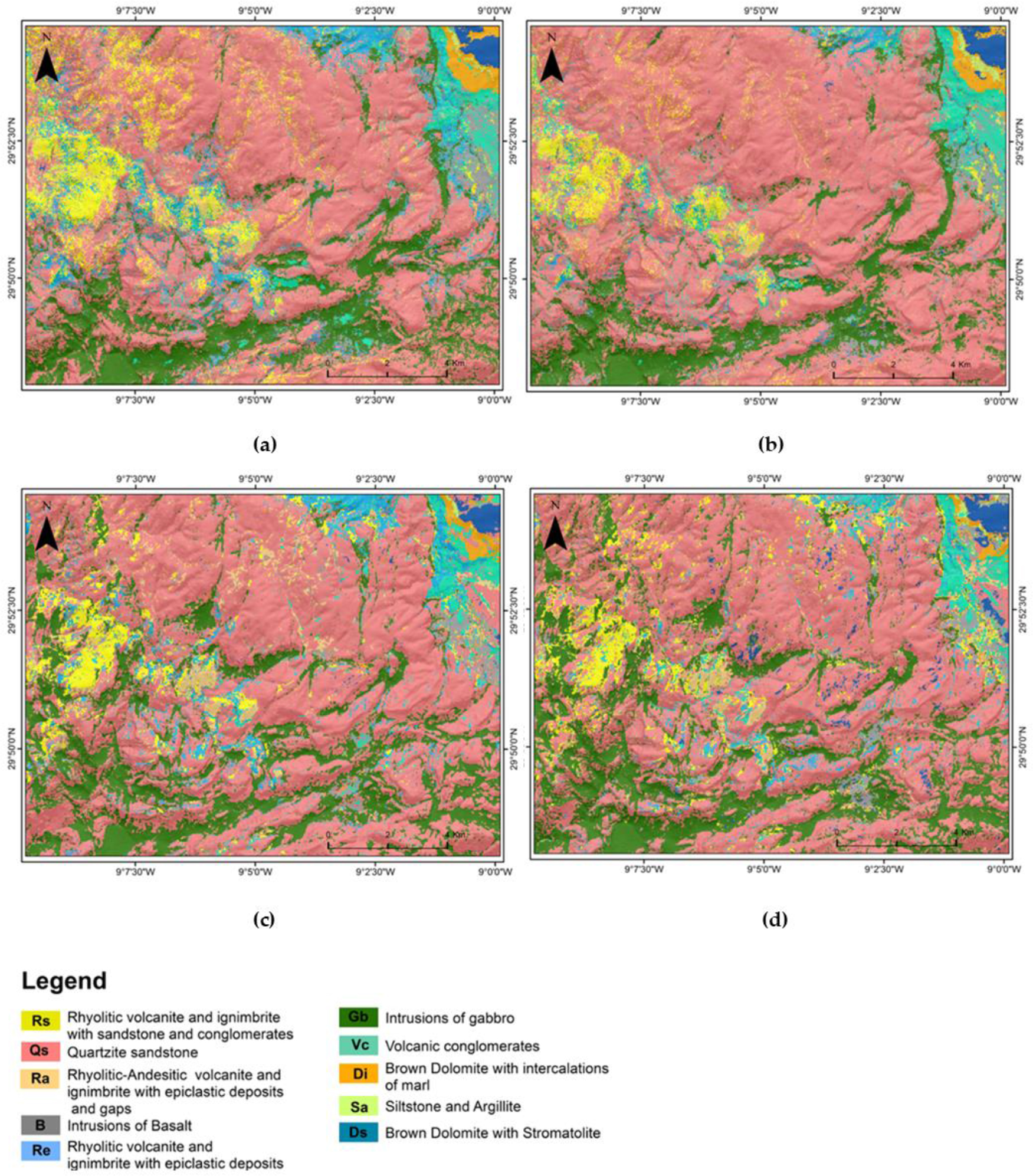
Figure 7.
Lithological classification maps: (a) MLC classification using ASTER image; (b) SVM classification using ASTER image; (c) MLC classification using OLI image; (d) SVM classification using OLI image
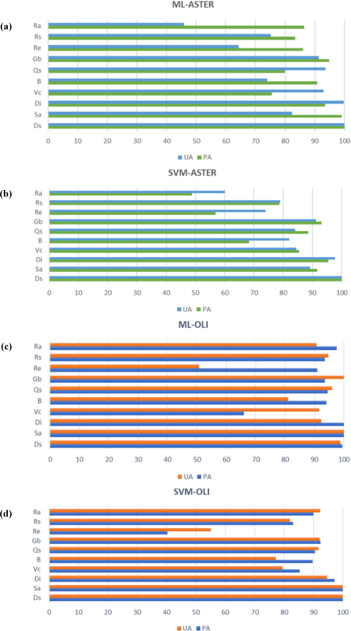
Figure 8.
User and producer accuracies: (a) ML ASTER; (b) SVM ASTER; (c) ML OLI; (d) SVM OLI
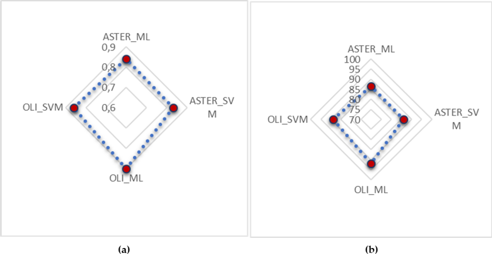
Figure 9.
Overall accuracy and Kappa coefficient of MLC and SVM classifications using ASTER and OLI: (a) overall accuracy; (b) Kappa coefficient
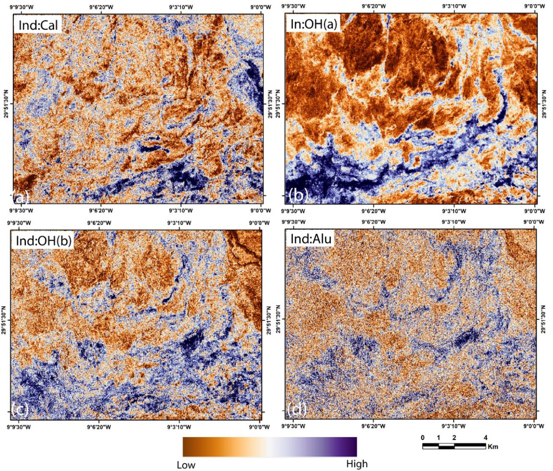
Figure 10.
Resulted images of the Ninomiya spectral indices: (a) Calcite; (b) OH(a); (c) OH(b); (d) Alunite
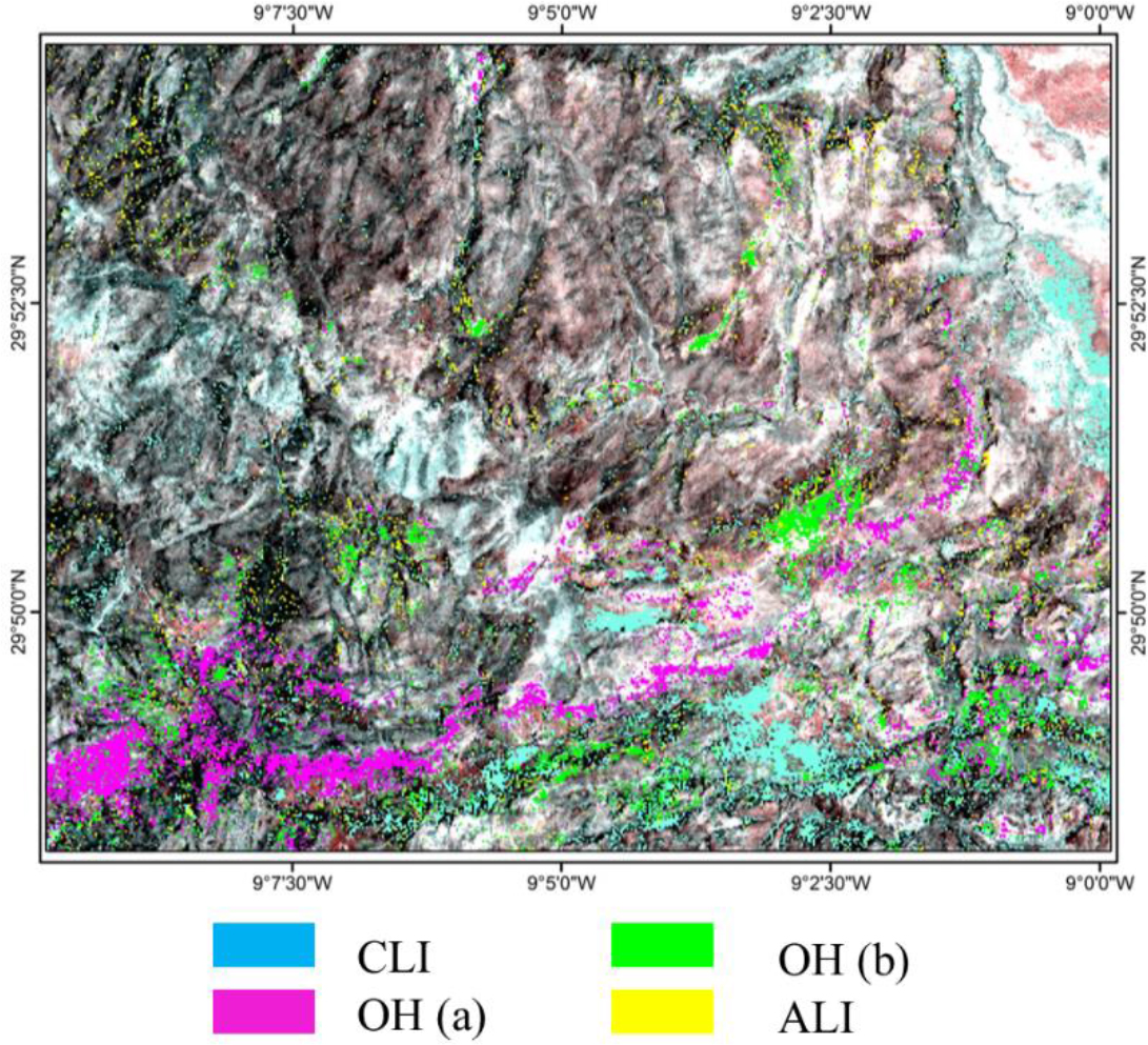
Figure 11.
Images of the Ninomiya spectral indices superimposed on the true color composite of ASTER image
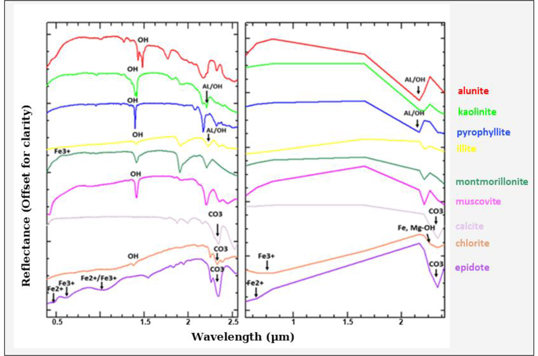
Figure 12.
Laboratory reflectance spectra of hydrothermal alteration minerals from USGS spectral library (left) and spectra resampled to ASTER bands (right)
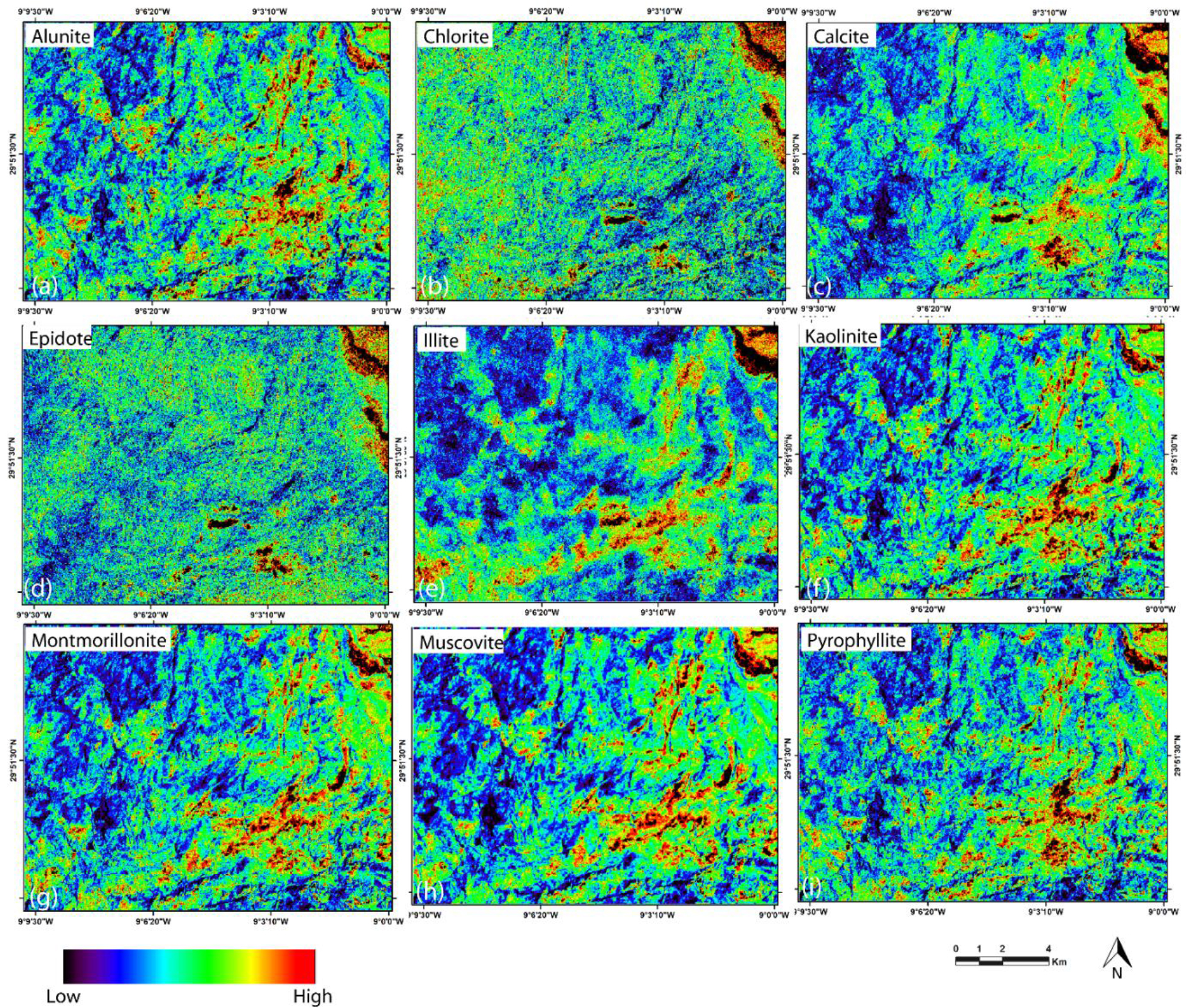
Figure 13.
ASTER resulting images of a high abundance of hydrothermal alteration minerals using CEM: (a) alunite; (b) chlorite; (c) calcite; (d) epidote; (e), illite; (f) kaolinite; (g), montmorillonite; (h) muscovite; (i) pyrophyllite
Table 5.
Selected end-member minerals (within the mapped hydrothermally altered zones) and USGS spectra matching scores computed using the SAM method and geographic coordinates
| Mineral | Score (%) | Geographical coordinates |
|---|---|---|
| Alunite | 81.6 | 29°51'3.56"N, 9°1'16.63"W |
| Calcite | 90.3 | 29°52'17.62"N, 9°0'13.03"W |
| Chlorite | 73.3 | 29°50'20.48"N, 9°4'16.54"W |
| Epidote | 80.2 | 29°49'18.45"N, 9°2'51.28"W |
| Illite | 89.3 | 29°54'35.83"N, 8°59'56.01"W |
| Kaolinite | 91.1 | 29°49'18.45"N, 9°2'51.28"W |
| Montmorillonite | 90.1 | 29°54'35.83"N, 8°59'56.01"W |
| Muscovite | 84.6 | 29°50'48.65"N, 9°2'38.17"W |
| Pyrophyllite | 74.1 | 29°51'7.29"N, 9°1'12.16"W |