
1. Introduction
Natural and artificial water reservoirs are currently facing significant degradation due to a combination of anthropogenic and environmental stressors (Yancheva et al., 2016; Mazur et al., 2024b). A primary concern is the global scale of eutrophication, which triggers excessive algal growth and harmful cyanobacterial blooms, leading to a rapid decline in water quality (Tomczyk et al., 2024). This phenomenon is frequently exacerbated by the inflow of nutrient-rich riverine waters and the accumulation of thick layers of organic sediments (Dondajewska-Pielka, 2024; Jakubiak et al., 2025). Furthermore, reservoirs located in urban or post-industrial areas are often affected by chemical contamination or high recreational pressure, which further compromises their ecological integrity (Starzec et al., 2024; Mazur et al., 2025). The consequences of such pollution are severe, including oxygen depletion, loss of biodiversity, and the overall deterioration of aquatic health (Mazurkiewicz et al., 2020; Biney et al., 2025). Consequently, active restoration and microbiological remediation have become necessary interventions to recover water homeostasis and maintain the functional roles of these ecosystems (Sitarek et al., 2017).
To address these challenges, restoration efforts employ a variety of physical, chemical, and biological methods, with microbiological remediation being increasingly favoured as a sustainable and non-invasive alternative (Mazur et al., 2024a; Tomczyk et al., 2024). This biotechnological approach relies on the application of specialized biopreparations, often composed of diverse microbial “cocktails” designed to accelerate the natural decomposition of organic matter and improve overall water quality (Mazurkiewicz et al., 2020; Dondajewska-Pielka, 2024; Jakubiak et al., 2025). Typical effective microorganisms (EM-type) preparations and other allochthonous microbial blends consist of synergistic consortia of microorganisms, including various lactic acid bacteria (e.g. Lactobacillus plantarum, L. casei, L. fermentum), photosynthetic bacteria (e.g. Rhodopseudomonas palustris), yeasts (Saccharomyces cerevisiae), and various Bacillus species (e.g. B. velezensis, B. licheniformis) (Javaid & Bajwa 2011; Sitarek et al., 2017; Mazur et al. 2024a; Zhu et al., 2026). These microorganisms secrete extracellular enzymes that break down complex organic sediments, thereby reducing sludge volume and nutrient concentrations while simultaneously increasing dissolved oxygen and water transparency (Kosov et al., 2018; Tomczyk et al., 2024; Mazur et al., 2025). By outcompeting harmful algae and pathogens for essential nutrients and space, these biopreparations help re-establish biological equilibrium and suppress cyanobacterial blooms (Mazurkiewicz et al., 2020; Jakubiak et al., 2025). Despite the documented efficacy of these microbial agents, the scientific literature reveals a notable research gap regarding their systemic safety for aquatic animals because existing studies are relatively scarce and often limited in scope (Tomczyk et al., 2024). These products are generally classified as safe for the environment; however, it is worth investigating whether the introduction of high concentrations of microbial biomass and metabolic by-products affects the physiological status of non-target aquatic organisms. Most studies prioritize water chemistry or microbial community structure, leaving a critical gap in our understanding of how these bioremediation tools affect the internal homeostasis and long-term health of vertebrate species. Recent experiments have attempted to address this issue by examining specific physiological responses in various models. For example, research on common carp (Cyprinus carpio) has focused on how these microbial additives influence growth performance and the micromorphometric parameters of vital organs, such as the gills and intestines (Jwher & Al-Sarhan, 2022). In juvenile Nile tilapia (Oreochromis niloticus), Xu et al. (2021) evaluated the effects of supplemental microbial diets on serum biochemical indices and the expression of appetite-regulating genes. Abdel-Aziz et al. (2020) showed that supplementing Nile tilapia diets with EM may lead to significant improvements in weight gain, specific growth rate, and survival, as well as better feed conversion efficiency. Similarly, dietary supplementation of the blunt snout bream (Megalobrama amblycephala) with EM has been shown to significantly enhance growth performance by increasing digestive enzyme activity and growth gene expression, while concurrently improving hepatic lipoprotein metabolism and reducing the risk of fatty liver (Zhu et al., 2026). Studies using the zebrafish (Danio rerio) have expanded this scope to include the spatial distribution of introduced strains and their impact on intestinal tissues. Ehsannia et al. (2022) indicated that probiotics may be helpful in fish farming. Even in invertebrates like the Chinese mitten crab (Eriocheir sinensis), such supplementation has been found to alter serum metabolite levels and intestinal microbiota (Li et al., 2024). Nevertheless, comprehensive evaluations combining multi-organ histology with physiological markers remain rare, emphasizing the need for further detailed assessments.
The common carp (Cyprinus carpio) is regarded as the oldest and most extensively domesticated fish species in history (Balon, 2004). It currently ranks fourth among freshwater species in global aquaculture production, a position attributed to its high reproductive rate, diverse feeding habits, and remarkable adaptability to fluctuating environmental conditions (Engin & Koşan, 2025). These characteristics, along with its rapid growth performance, make it a central component of freshwater farming systems worldwide (Rahman, 2015). In addition to its commercial value, the common carp has become a fundamental model for aquatic toxicology and ecological monitoring (Yancheva et al., 2022). This species is frequently employed to evaluate the biological effects of various chemical pollutants and environmental stressors (Gül et al., 2012; Yancheva et al., 2016, 2026; Bojarski et al., 2022, 2024; Arslan et al., 2023; Mancera-Rodríguez et al., 2024; Gül et al., 2025; Farooq et al., 2026). The reliability of toxicological data in laboratory settings depends heavily on the standardisation of test subjects to ensure the reproducibility of results. The C. carpio R3R8 genetic line is one of the well-established models used for this purpose (Rakus et al., 2012). The high genetic homogeneity of this line minimizes individual variation in physiological and immune responses (Kolder et al., 2016). The R3R8 model is frequently used to study immune system dynamics, disease susceptibility, and the impact of acute stress (Engelsma et al., 2003; Gaafar et al., 2011). Utilising such a standardised genetic model is essential for the precise assessment of how modern biopreparations influence fish homeostasis under controlled experimental conditions.
We hypothesized that exposure of common carp to the commercial biological preparations ACS AQUAQULTURE 1.0, 2.0, and 3.0 at the applied concentration (1.5 ml/l) would not induce significant physiological or histopathological effects. Specifically, we assumed that the tested biopreparations would not disrupt haematological and biochemical parameters, impair haematopoietic activity, or cause alterations in the microstructure of gills, liver, trunk kidney, and intestine, thereby confirming their safety for use in sustainable aquaculture and bioremediation of aquatic ecosystems. To verify the hypothesis, blood analyses (haematological and biochemical determinations), assessments of haematopoietic activity, and histopathological examinations of vital organs were conducted to detect potential functional and structural changes. The expected outcome is a clearer understanding of the safety profile of the tested additives.
2. Material and methods
2.1. Experimental design
The study was approved by the Local Ethics Committee for Animal Testing at the Medical University of Silesia in Katowice (Resolution No. 13/2023 of 24.05.2023). Clinically healthy, sexually immature common carp (C. carpio) of the R3R8 line were used, maintained under laboratory conditions. The fish weighed 70–80 g, with a total length of 16–17 cm. The experiment was conducted at the Institute of Ichthyobiology and Aquaculture of the Polish Academy of Sciences in Gołysz (Zaborze, Poland). Fish were distributed across eight tanks, with ten individuals per tank (total n = 80). Each tank had a volume of 300 l and contained 200 l of water. Following a 14-day acclimation period, four groups were established: one control and three experimental (A1, A2, A3). Each group consisted of two tanks with 10 fish per tank. Fish from group A1 were exposed to ACS AQUAQULTURE 1.0 preparation, fish from group A2 to ACS AQUAQULTURE 2.0, and fish from group A3 to ACS AQUAQULTURE 3.0. According to information provided by the manufacturer, ACS Poland, ACS AQUAQULTURE 1.0 is a preparation obtained through the fermentation of fruit concentrates. It is used in fish culture to, for example, improve feed utilisation. ACS AQUAQULTURE 2.0 is a preparation produced from fruit concentrates, barley straw, and alder cones. In fish farming, it is applied, for example, to protect the mucous membranes and roe against fungal growth. The preparation reduces the water pH. ACS AQUAQULTURE 3.0 is produced from molasses and a mixture of herbs (wild garlic, basil, oregano, moringa, green tea). It is used in aquaculture to limit the development of bacterial, viral, and fungal pathogens. The aforementioned preparations support fish immunity and limit the accumulation of organic substances in the water. They contain Terra Biosa bacterial cultures. For each experimental group, the concentration of the tested preparation was 1.5 ml/l of water. This concentration was selected after consultation with the manufacturer, who identified the range of 1.5–2 ml/l as the highest concentration recommended for the bioremediation of water reservoirs. The exposure lasted 7 or 14 days.
2.2. Experimental conditions
During both acclimation and exposure, water in all tanks was renewed twice a day. In the exposure phase, the appropriate amount of the tested preparations was added to the experimental tanks immediately after each water change. Water temperature and dissolved oxygen were measured with an Oxi 3310 oximeter (WTW, Poland), and pH with a pH meter (Mettler Toledo, Switzerland). Concentrations of ammonia, nitrites, nitrates, as well as general hardness and carbonate hardness, were determined using colorimetric test kits (Zoolek, Łódź, Poland). Physicochemical parameters were monitored at 2-day intervals. The parameters are presented in Table 1.
Table 1
Water parameters (mean value ± SD) in the control and experimental groups
| Parameter | Control | A1 | A2 | A3 |
|---|---|---|---|---|
| Temp. (°C) | 20.63 ± 0.17 | 20.53 ± 0.15 | 20.61 ± 0.10 | 20.65 ± 0.17 |
| O2 (mg/l) | 6.91 ± 0.67 | 6.83 ± 0.51 | 6.74 ± 0.49 | 6.89 ± 0.60 |
| pH | 7.22 ± 0.09 | 7.08 ± 0.14 | 7.11 ± 0.13 | 7.14 ± 0.12 |
| NH3 (mg/l) | 0.01 ± 0.00 | 0.01 ± 0.00 | 0.01 ± 0.00 | 0.01 ± 0.00 |
| NO2 − (mg/l) | 0.12 ± 0.14 | 0.14 ± 0.31 | 0.23 ± 0.38 | 0.27 ± 0.41 |
| NO3 − (mg/l) | 4.86 ± 2.57 | 4.86 ± 3.23 | 5.36 ± 3.32 | 4.71 ± 2.79 |
| GH (dGH) | 4.14 ± 0.36 | 4.21 ± 0.43 | 4.43 ± 0.65 | 4.14 ± 0.36 |
| KH (dKH) | 3.00 ± 0.00 | 3.00 ± 0.00 | 3.00 ± 0.00 | 3.00 ± 0.00 |
GH – general hardness; KH – carbonate hardness.
2.3. Biological material collection
After 7 and 14 days of exposure, biological samples were collected for haematological, biochemical, haematopoietic, and histopathological analyses. Without the use of anaesthesia in order to avoid its influence on haematological and plasma biochemical parameters, blood was taken from the caudal vein into heparinized Eppendorf tubes (Heparinum WZF, Polfa, Poland). A portion of the blood was used for haematological analysis, while the remainder was centrifuged (3,000 × g, 20 min) to obtain plasma, which was stored at −80°C until biochemical assays. After blood collection, fish were euthanized with an overdose of MS-222 (Merck, USA; 500 mg/l). Next, the head kidney was collected for the preparation of smears. Gills, liver, and trunk kidney were sampled and preserved in 4% buffered formaldehyde.
2.4. Haematological and plasma biochemical analyses
Red and white blood cell counts were determined by diluting blood 100-fold with Hayem’s solution (Chempur, Poland) and cells were counted using a Bürker haemocytometer under a standard optical microscope. Haematocrit (Ht) was measured after centrifuging blood-filled capillary tubes at 16,000 × g for 5 min using a Haematokrit 200 centrifuge (Hettich, Germany). Haemoglobin (Hb) concentration was assessed by mixing blood 1:250 with Drabkin’s reagent (Chempur, Poland) and measuring absorbance at 540 nm (UV-1601PC spectrophotometer, Shimadzu, Japan). Derived erythrocyte indices (mean corpuscular volume, MCV; mean corpuscular haemoglobin, MCH; mean corpuscular haemoglobin concentration, MCHC) were calculated using standard formulas. Blood biochemical analyses were conducted at a veterinary laboratory “Vetlab” (Katowice, Poland) and included measurements of glucose (Glu), total protein (TP), triglyceride (Tg) concentrations, and aspartate aminotransferase (AST) and alkaline phosphatase (ALP) activity. The above-mentioned biochemical indicators were measured using an AU680 analyser (Beckman Coulter, USA).
2.5. Haematopoietic analysis
Head kidneys were isolated, and haematopoietic tissue preparations were made. The smears were stained with May–Grünwald and Giemsa solutions. Percentages of all types of haematopoietic precursor cells were determined by examining 500 cells in each smear. Identification of particular cell types was based on the morphological features described by Fijan (2002) and Kondera (2011). Due to their morphological similarity, early blast cells from different lineages were pooled to minimize identification bias. Cells with unclear characteristics were classified as “unclassified cells.”
2.6. Histological analysis
Tissue samples for histological examination were collected from six individuals per group at each designated sampling point. Samples of the selected organs – gills, liver, trunk kidney, and intestine – were fixed in 4% buffered formaldehyde (Chempur, Poland) for 2 weeks. Following fixation, the samples were embedded in Paraplast Regular (Sigma, St. Louis, MO, USA). Transverse sections of 6 μm thickness were obtained using a Zeiss Hyrax M55 microtome, mounted onto glass slides, and subjected to haematoxylin and eosin (H + E) staining. The sections were stained with Delafield’s haematoxylin for 5 min, rinsed in tap water, and counterstained with eosin for 5 min to visualize general cytological features.
The slides were evaluated in a blinded manner using a Nikon Eclipse E600 light microscope. Digital micrographs were captured with a Nikon DS-Fi1c camera and analysed using NIS-Elements F software. The histological assessment focused on the overall tissue architecture of the examined organs and the detection of any pathological alterations. Particular attention was paid to the histopathological changes described by Bernet et al. (1999).
2.7. Statistical analysis
The first step of the statistical analysis was to test whether the experimental data followed a normal distribution. This was done using the Shapiro–Wilk test. The homogeneity of variances was evaluated using Levene’s test. Based on the results of these tests, a decision was made whether to use parametric tests (one-way ANOVA followed by Tukey’s HSD post hoc test if the ANOVA returned p-value < 0.05) or non-parametric tests (Kruskal–Wallis test followed by Dunn’s post hoc test if the Kruskal–Wallis test returned p-value < 0.05). The level of significance for all tests performed was set at 0.05.
Parametric tests were applied to haematological and biochemical data. Non-parametric tests were used for the haematopoietic data. The statistical analysis was performed using R software (version 4.5.1). The detailed results of the statistical analysis are presented in Section 3. Letter symbols indicate the presence or absence of statistically significant differences.
3. Results
3.1. Haematological parameters
In terms of haematological parameters (Tables 2–3), the ANOVA test rejected the null hypothesis of equal MCHC after 14 days of exposure (p = 0.025). The post hoc test showed a significant difference between group A2 and the control group. This difference was statistically significant at p adj = 0.033. The test did not reveal other differences among the groups.
Table 2
Haematological parameters after 7 days of exposure to ACS AQUAQULTURE preparations (mean value ± SD)
| Parameter | Control | A1 | A2 | A3 |
|---|---|---|---|---|
| RBC (106/µL) | 1.36 ± 0.16 | 1.21 ± 0.30 | 1.21 ± 0.19 | 1.24 ± 0.11 |
| Ht (%) | 25.28 ± 2.26 | 25.45 ± 2.05 | 26.68 ± 2.11 | 25.43 ± 4.18 |
| Hb (g/dl) | 6.59 ± 0.49 | 6.75 ± 0.58 | 6.96 ± 0.51 | 6.83 ± 1.12 |
| MCV (fl) | 188.83 ± 30.47 | 219.58 ± 44.71 | 225.55 ± 40.01 | 205.99 ± 29.54 |
| MCH (pg) | 49.04 ± 5.50 | 58.32 ± 12.40 | 59.07 ± 12.28 | 55.34 ± 7.88 |
| MCHC (g/dl) | 26.14 ± 1.39 | 26.53 ± 0.72 | 26.13 ± 1.49 | 26.91 ± 1.73 |
| WBC (103/µL) | 24.10 ± 3.92 | 27.05 ± 4.87 | 23.98 ± 3.21 | 23.23 ± 2.70 |
No statistically significant differences occurred.
RBC – red blood cell count; Ht – haematocrit value; Hb – haemoglobin concentration; MCV – mean corpuscular volume; MCH – mean corpuscular haemoglobin; MCHC – mean corpuscular haemoglobin concentration; WBC – white blood cell count.
Table 3
Haematological parameters after 14 days of exposure to ACS AQUAQULTURE preparations (mean value ± SD)
| Parameter | Control | A1 | A2 | A3 |
|---|---|---|---|---|
| RBC (106/µL) | 1.39 ± 0.18 | 1.31 ± 0.22 | 1.47 ± 0.27 | 1.44 ± 0.26 |
| Ht (%) | 25.00 ± 2.90 | 25.75 ± 1.95 | 25.18 ± 1.64 | 24.75 ± 1.98 |
| Hb (g/dl) | 7.00 ± 1.06 | 7.02 ± 0.52 | 6.55 ± 0.39 | 6.65 ± 0.48 |
| MCV (fl) | 181.58 ± 26.64 | 202.24 ± 39.06 | 175.94 ± 33.13 | 177.83 ± 39.37 |
| MCH (pg) | 50.91 ± 9.50 | 55.40 ± 12.42 | 45.77 ± 8.62 | 48.08 ± 11.83 |
| MCHC (g/dl) | 27.92 ± 1.49A | 27.32 ± 1.56AB | 26.04 ± 1.13B | 26.92 ± 1.08AB |
| WBC (103/µL) | 23.48 ± 5.96 | 23.15 ± 4.25 | 24.13 ± 2.92 | 24.33 ± 5.26 |
Different letters in a row indicate that the corresponding values are statistically significantly different (p adj < 0.05).
RBC – red blood cell count; Ht – haematocrit value; Hb – haemoglobin concentration; MCV – mean corpuscular volume; MCH – mean corpuscular haemoglobin; MCHC – mean corpuscular haemoglobin concentration; WBC – white blood cell count.
3.2. Haematopoietic parameters
Regarding haematopoietic parameters (Tables 4–5), the Kruskal–Wallis test rejected the null hypothesis of equal percentage of monocytoid cells after 14 days of exposure (p = 0.034). However, the post hoc test did not show significant differences.
Table 4
Haematopoietic parameters in common carp (Cyprinus carpio) after 7 days of exposure to ACS AQUAQULTURE preparations (mean value ± SD)
| Parameter | Control | A1 | A2 | A3 |
|---|---|---|---|---|
| Early blast cells (%) | 6.72 ± 1.23 | 6.40 ± 1.65 | 6.08 ± 2.55 | 6.68 ± 1.52 |
| Neutrophilic cells (%) | 14.30 ± 2.87 | 13.80 ± 3.29 | 14.72 ± 2.88 | 13.66 ± 2.79 |
| Neutrophilic myelocytes (%) | 5.28 ± 2.48 | 5.06 ± 1.73 | 6.12 ± 3.71 | 4.52 ± 2.10 |
| Neutrophilic metamyelocytes (%) | 4.56 ± 3.87 | 4.34 ± 2.90 | 4.42 ± 1.80 | 4.62 ± 2.63 |
| Band neutrophils (%) | 2.24 ± 1.68 | 2.14 ± 1.03 | 1.98 ± 0.97 | 2.24 ± 1.23 |
| Segmented neutrophils (%) | 2.22 ± 1.07 | 2.26 ± 1.01 | 2.20 ± 1.51 | 2.28 ± 1.05 |
| Monocytoid cells (%) | 1.26 ± 0.68 | 1.38 ± 0.24 | 1.16 ± 0.51 | 1.30 ± 0.34 |
| Promonocytes (%) | 0.54 ± 0.40 | 0.64 ± 0.51 | 0.66 ± 0.46 | 0.66 ± 0.43 |
| Monocytes (%) | 0.72 ± 0.59 | 0.74 ± 0.37 | 0.50 ± 0.38 | 0.64 ± 0.35 |
| Lymphoid cells (%) | 62.14 ± 5.06 | 62.68 ± 4.61 | 61.10 ± 5.27 | 62.20 ± 4.32 |
| Prolymphocytes (%) | 2.16 ± 2.59 | 2.40 ± 1.01 | 1.98 ± 1.01 | 3.16 ± 2.99 |
| Lymphocytes (%) | 58.90 ± 7.62 | 59.18 ± 4.43 | 58.10 ± 4.90 | 57.56 ± 6.73 |
| Proplasmocytes (%) | 0.38 ± 0.45 | 0.46 ± 0.41 | 0.52 ± 0.45 | 0.76 ± 0.47 |
| Plasmocytes (%) | 0.70 ± 0.54 | 0.64 ± 0.46 | 0.50 ± 0.44 | 0.72 ± 0.29 |
| Erythroid cells (%) | 5.86 ± 0.87 | 5.68 ± 1.24 | 5.82 ± 1.83 | 5.08 ± 1.39 |
| Basophilic erythroblasts (%) | 0.80 ± 0.66 | 1.04 ± 1.05 | 1.12 ± 0.73 | 1.08 ± 0.84 |
| Polychromatophilic erythroblasts (%) | 1.08 ± 0.59 | 0.80 ± 0.66 | 1.18 ± 0.82 | 0.70 ± 0.40 |
| Orthochromatic erythroblasts (%) | 0.96 ± 0.59 | 0.36 ± 0.37 | 0.86 ± 0.68 | 0.64 ± 0.62 |
| Erythrocytes (%) | 1.52 ± 0.88 | 2.04 ± 1.71 | 1.32 ± 0.71 | 1.40 ± 0.52 |
| Juvenile erythrocytes (%) | 1.50 ± 0.71 | 1.44 ± 0.84 | 1.34 ± 0.74 | 1.26 ± 0.67 |
| Basophilic cells (%) | 3.68 ± 1.18 | 4.58 ± 1.04 | 4.14 ± 2.05 | 5.00 ± 1.52 |
| Basophilic progranulocytes (%) | 0.94 ± 0.65 | 1.08 ± 0.83 | 1.20 ± 1.15 | 1.38 ± 0.99 |
| Basophilic metagranulocytes (%) | 0.78 ± 0.82 | 1.26 ± 0.85 | 0.94 ± 1.03 | 1.62 ± 0.77 |
| Juvenile basophils (%) | 0.94 ± 0.53 | 1.34 ± 1.02 | 1.14 ± 0.93 | 0.74 ± 0.57 |
| Basophils (%) | 1.02 ± 0.53 | 0.90 ± 0.52 | 0.86 ± 0.50 | 1.26 ± 0.27 |
| Eosinophils (%) | 0.22 ± 0.24 | 0.08 ± 0.14 | 0.08 ± 0.10 | 0.14 ± 0.13 |
| Thrombocytes (%) | 3.94 ± 2.18 | 3.44 ± 1.81 | 4.48 ± 1.42 | 3.68 ± 1.87 |
| Unclassified (%) | 1.88 ± 0.94 | 1.96 ± 1.22 | 2.42 ± 1.53 | 2.26 ± 1.15 |
No statistically significant differences occurred.
Table 5
Haematopoietic parameters in common carp (Cyprinus carpio) after 14 days of exposure to ACS AQUAQULTURE preparations (mean value ± SD)
| Parameter | Control | A1 | A2 | A3 |
|---|---|---|---|---|
| Early blast cells (%) | 6.28 ± 1.46 | 5.74 ± 1.62 | 5.98 ± 1.53 | 6.04 ± 1.48 |
| Neutrophilic cells (%) | 15.62 ± 3.17 | 13.88 ± 2.74 | 13.78 ± 2.86 | 14.88 ± 3.54 |
| Neutrophilic myelocytes (%) | 5.26 ± 2.82 | 4.70 ± 1.75 | 5.92 ± 3.12 | 4.74 ± 2.17 |
| Neutrophilic metamyelocytes (%) | 5.96 ± 2.97 | 4.98 ± 2.77 | 3.84 ± 2.48 | 4.66 ± 2.13 |
| Band neutrophils (%) | 2.18 ± 0.75 | 2.12 ± 0.85 | 2.44 ± 1.29 | 2.76 ± 0.88 |
| Segmented neutrophils (%) | 2.22 ± 1.14 | 2.08 ± 0.97 | 1.58 ± 0.77 | 2.72 ± 1.13 |
| Monocytoid cells (%) | 1.50 ± 0.43 | 1.02 ± 0.49 | 1.08 ± 0.27 | 1.20 ± 0.25 |
| Promonocytes (%) | 0.74 ± 0.54 | 0.58 ± 0.36 | 0.46 ± 0.45 | 0.54 ± 0.35 |
| Monocytes (%) | 0.76 ± 0.39 | 0.44 ± 0.23 | 0.62 ± 0.38 | 0.66 ± 0.37 |
| Lymphoid cells (%) | 60.44 ± 3.60 | 63.44 ± 4.83 | 64.58 ± 4.58 | 62.04 ± 5.03 |
| Prolymphocytes (%) | 2.40 ± 1.00 | 1.98 ± 1.88 | 1.64 ± 1.15 | 2.08 ± 1.77 |
| Lymphocytes (%) | 56.94 ± 4.06 | 59.88 ± 4.24 | 61.36 ± 4.33 | 58.48 ± 4.12 |
| Proplasmocytes (%) | 0.48 ± 0.47 | 0.86 ± 0.66 | 0.98 ± 0.77 | 0.86 ± 0.57 |
| Plasmocytes (%) | 0.62 ± 0.57 | 0.72 ± 0.38 | 0.60 ± 0.34 | 0.62 ± 0.38 |
| Erythroid cells (%) | 5.02 ± 1.04 | 5.58 ± 1.05 | 5.02 ± 1.60 | 5.38 ± 1.70 |
| Basophilic erythroblasts (%) | 1.00 ± 0.57 | 0.66 ± 0.63 | 0.52 ± 0.51 | 0.68 ± 0.52 |
| Polychromatophilic erythroblasts (%) | 0.76 ± 0.74 | 0.76 ± 0.84 | 0.82 ± 0.61 | 0.70 ± 0.58 |
| Orthochromatic erythroblasts (%) | 0.52 ± 0.43 | 0.78 ± 0.63 | 0.92 ± 0.66 | 0.88 ± 0.62 |
| Erythrocytes (%) | 1.62 ± 0.79 | 1.68 ± 0.69 | 1.50 ± 0.85 | 1.58 ± 0.92 |
| Juvenile erythrocytes (%) | 1.12 ± 0.81 | 1.70 ± 0.74 | 1.26 ± 0.85 | 1.54 ± 0.85 |
| Basophilic cells (%) | 5.26 ± 2.41 | 4.18 ± 1.41 | 4.54 ± 1.85 | 5.00 ± 2.23 |
| Basophilic progranulocytes (%) | 1.68 ± 1.26 | 0.92 ± 0.65 | 1.34 ± 1.31 | 1.38 ± 1.11 |
| Basophilic metagranulocytes (%) | 1.32 ± 1.23 | 1.24 ± 0.84 | 1.24 ± 1.04 | 1.40 ± 1.02 |
| Juvenile basophils (%) | 1.10 ± 0.58 | 1.06 ± 1.24 | 0.92 ± 0.76 | 1.08 ± 0.75 |
| Basophils (%) | 1.16 ± 0.35 | 0.96 ± 0.62 | 1.04 ± 0.79 | 1.14 ± 0.77 |
| Eosinophils (%) | 0.10 ± 0.11 | 0.10 ± 0.14 | 0.08 ± 0.14 | 0.12 ± 0.17 |
| Thrombocytes (%) | 3.94 ± 1.86 | 3.56 ± 1.53 | 2.76 ± 1.39 | 2.76 ± 1.51 |
| Unclassified (%) | 1.84 ± 1.28 | 2.50 ± 1.85 | 2.18 ± 0.99 | 2.58 ± 2.20 |
No statistically significant differences occurred.
3.3. Plasma biochemical parameters
With respect to plasma biochemical parameters (Tables 6–7), the ANOVA test revealed statistically significant differences in Glu concentration after 14 days of exposure (p = 0.015). The post hoc test showed that p adj for the comparison between group A1 and the control group was equal to 0.05, i.e. at the borderline of significance. The ANOVA test rejected the null hypothesis of equal TP concentrations after 14 days of exposure (p = 0.029). The post hoc test showed that, with regard to this parameter, group A1 differed significantly from group A3. This difference was statistically significant at p adj = 0.038. The test did not reveal other differences among the groups.
Table 6
Plasma biochemical parameters after 7 days of exposure to ACS AQUAQULTURE preparations (mean value ± SD)
| Parameter | Control | A1 | A2 | A3 |
|---|---|---|---|---|
| Glu (mmol/l) | 4.41 ± 1.03 | 4.25 ± 1.21 | 4.90 ± 1.31 | 4.95 ± 1.38 |
| TP (g/l) | 22.53 ± 1.51 | 23.63 ± 2.35 | 21.24 ± 2.86 | 21.79 ± 3.22 |
| Tg (mmol/l) | 1.74 ± 0.25 | 1.65 ± 0.23 | 1.64 ± 0.17 | 1.55 ± 0.21 |
| AST (U/l) | 114.42 ± 31.16 | 138.52 ± 59.80 | 162.55 ± 55.70 | 149.96 ± 54.83 |
| ALP (U/l) | 127.00 ± 52.51 | 134.80 ± 70.53 | 132.50 ± 69.23 | 122.90 ± 57.85 |
No statistically significant differences occurred.
Glu – glucose; TP – total protein; Tg – triglycerides; AST – aspartate aminotransferase; ALP – alkaline phosphatase.
Table 7
Plasma biochemical parameters after 14 days of exposure to ACS AQUAQULTURE preparations (mean value ± SD)
| Parameter | Control | A1 | A2 | A3 |
|---|---|---|---|---|
| Glu (mmol/l) | 4.74 ± 0.83 | 3.63 ± 0.84 | 4.43 ± 0.74 | 3.89 ± 0.77 |
| TP (g/l) | 22.48 ± 2.36 AB | 22.81 ± 1.97 A | 20.45 ± 3.15 AB | 20.01 ± 2.09 B |
| Tg (mmol/l) | 1.68 ± 0.30 | 1.63 ± 0.20 | 1.51 ± 0.26 | 1.45 ± 0.34 |
| AST (U/l) | 115.49 ± 30.35 | 109.15 ± 24.98 | 93.13 ± 11.15 | 103.07 ± 21.92 |
| ALP (U/l) | 160.50 ± 28.91 | 150.50 ± 99.80 | 140.70 ± 92.47 | 195.30 ± 99.08 |
Different letters in a row indicate that the corresponding values are statistically significantly different (p adj < 0.05).
Glu – glucose; TP – total protein; Tg – triglycerides; AST – aspartate aminotransferase; ALP – alkaline phosphatase.
3.4. Histological analysis
Histological images of the examined organs are shown in Figures 1–4. In general, in all tested organs (gills, liver, trunk kidney, and intestine), the histological architecture was consistent with that typically described for common carp, demonstrating normal cellular morphology and intact tissue integrity. Importantly, no degenerative, inflammatory, or other pathological alterations were observed in either the control or experimental groups.
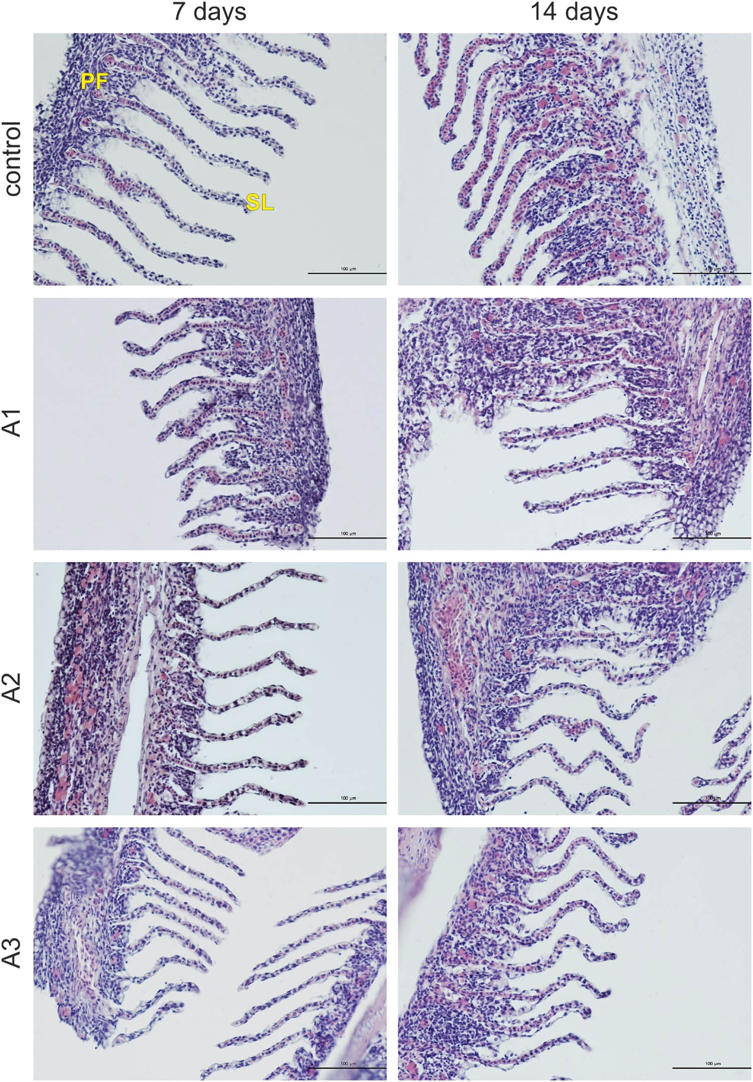
Figure 1
Photomicrographs of the gills of the common carp in the control and experimental groups. PF – primary filament; SL – secondary lamellae. H + E staining. Scale bars: 100 μm.
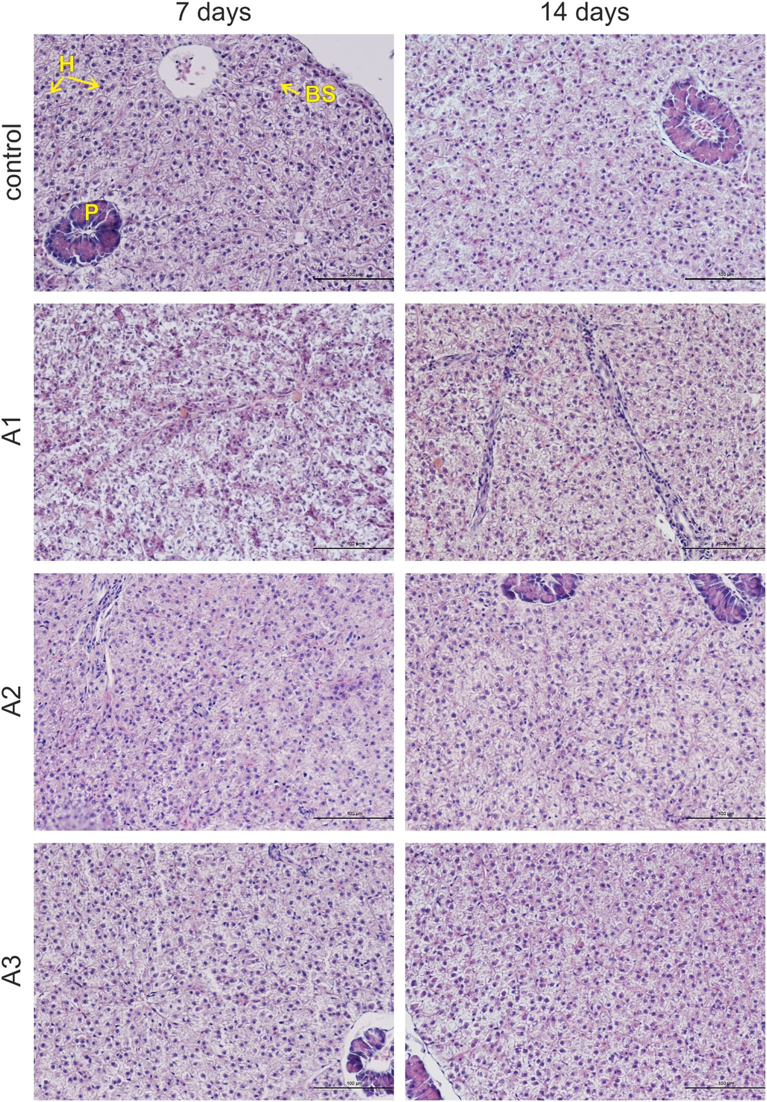
Figure 2
Photomicrographs of the livers of the common carp in the control and experimental groups. H – hepatocytes; BS – blood sinusoid; P – pancreas. H + E staining. Scale bars: 100 μm.
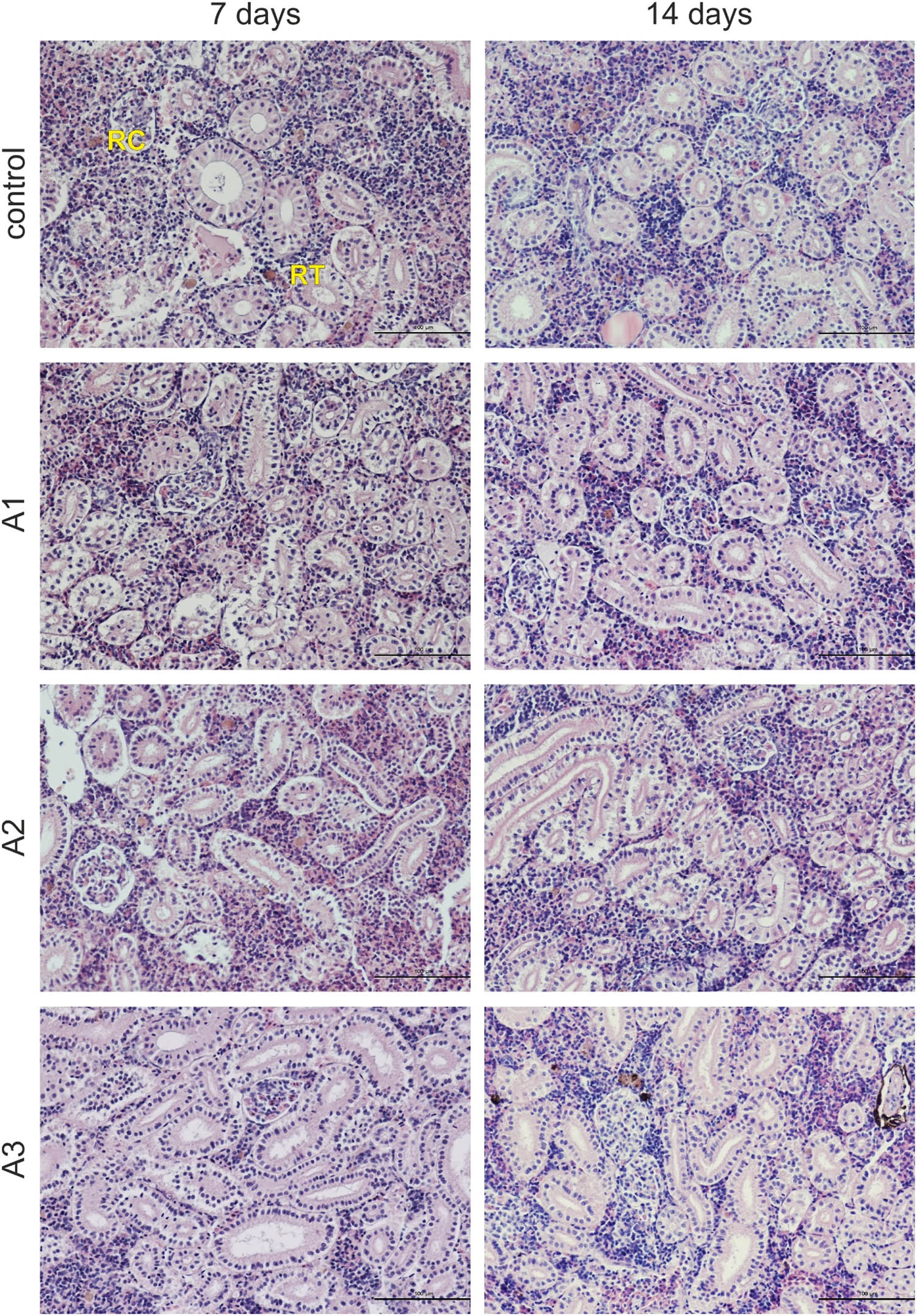
Figure 3
Photomicrographs of the trunk kidneys of the common carp in the control and experimental groups. RC – renal corpuscle; RT – renal tubule. H + E staining. Scale bars: 100 μm.
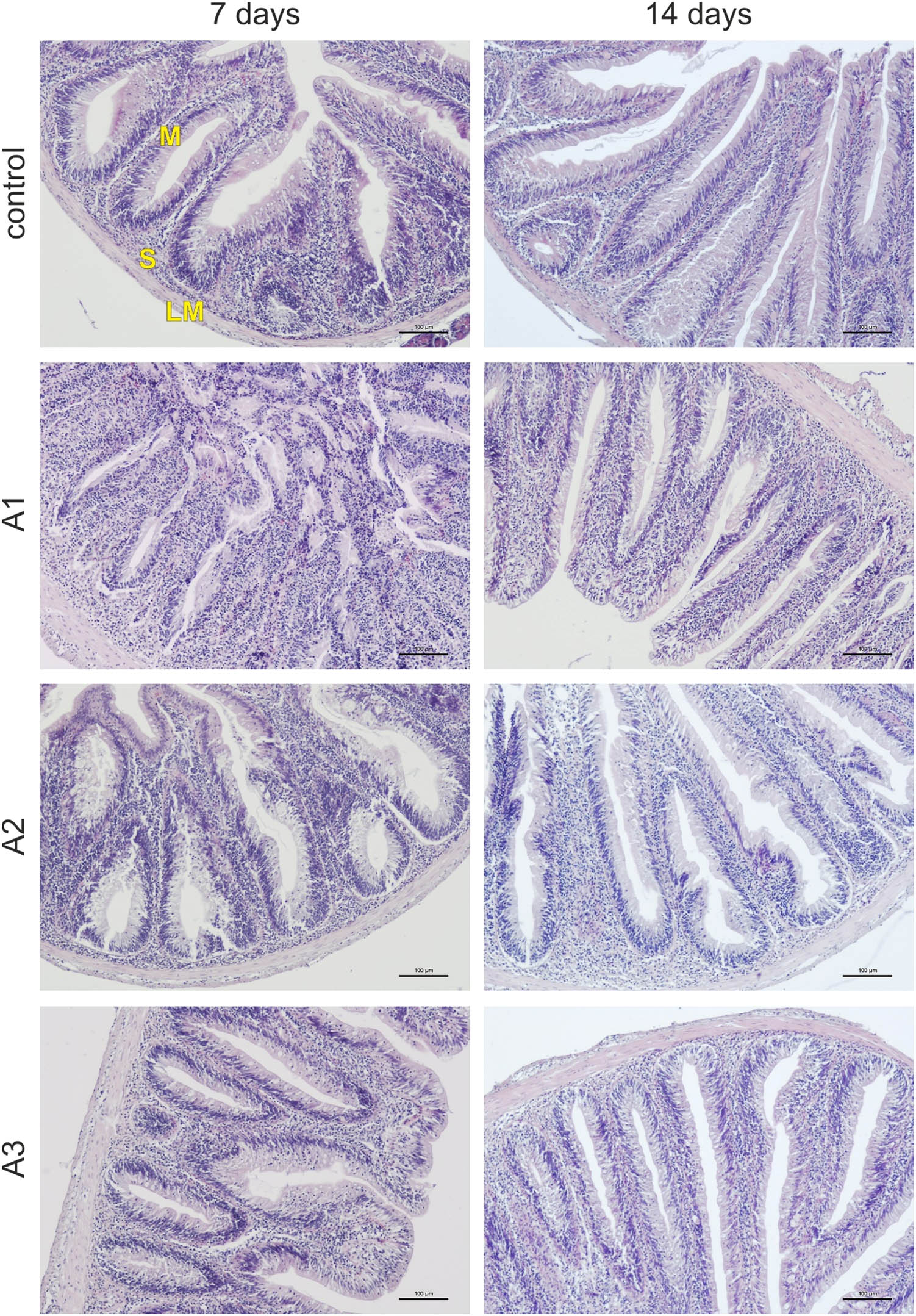
Figure 4
Photomicrographs of the intestines of the common carp in the control and experimental groups. LM – lamina muscularis; S – submucosa; M – mucosa. H + E staining. Scale bars: 100 μm.
4. Discussion
With respect to the haematological, haematopoietic, and biochemical parameters examined in the present study, the only statistically significant change observed between the control group and the experimental groups was a decrease in MCHC in group A2. However, in our opinion, as the value observed in group A2 (26.04 ± 1.13 g/dl) was within the reference interval reported by Witeska et al. (2016) (25.66–28.49 g/dl), the above-mentioned change, although statistically significant, is not biologically or toxicologically relevant. This conclusion is supported by the fact that it is the only statistically significant change among the above-mentioned parameters.
Histological analysis of the gills, liver, trunk kidney, and intestine revealed no pathological changes. Considering the results of all analyses conducted in the present study, the tested preparations can be preliminarily regarded as safe for common carp. However, this conclusion should be confirmed in further studies, e.g. experiments including other lineages of common carp as well as fish with body mass and length different from those used in the present study. Moreover, the effects of various physicochemical water parameters, exposure durations longer than 14 days, and different doses of the examined preparations should be assessed in further investigations.
The beneficial effect of microbiological preparations on fish has been demonstrated by some researchers. For example, Hendam et al. (2023) found that the probiotic Pediococcus acidilactici, as a water additive, improved water quality, enhanced the expression of immune regulatory genes, and led to a higher survival rate during an Aspergillus flavus challenge in Nile tilapia (Oreochromis niloticus). Moreover, Redhwan et al. (2024) showed that a water-applied probiotic containing Bacillus sp., Pediococcus sp., and Enterococcus sp. improved water quality, enhanced growth performance and feed utilisation, and reduced mortality during an Aeromonas sobria challenge in fish of the same species. Nassar et al. (2025) revealed that the addition of Bacillus subtilis and Bacillus licheniformis probiotics to the water improved the growth and health of gilt-head seabream (Sparus aurata) by regulating the immune responses and antioxidant status. Tarnecki et al. (2019) showed that probiotic benefits include accelerated gastrointestinal tract development, enhanced immunity, and inhibition of opportunistic bacteria. According to Fachri et al. (2024), the diverse beneficial effects exhibited by various probiotic strains, including Arthrobacter, Bacillus, Lactobacillus, Bifidobacterium, and Clostridium, are associated with promoting growth, enhancing resistance to bacterial, viral, and parasitic diseases, reducing stress, improving water quality, and supporting environmental sustainability.
5. Conclusion
Microbial preparations are increasingly used due to their various beneficial effects on the aquatic environment. However, relatively few studies have focused on the safety of such products for fish and their potential toxic effects on aquatic organisms. The present study demonstrated that the tested commercial biological preparations (ACS AQUAQULTURE 1.0, 2.0, and 3.0) do not induce adverse effects in common carp and can therefore be considered safe for fish of this species. Nevertheless, further studies are recommended to confirm this conclusion.
Funding information
Authors state no funding involved.
Author contributions
Conceptualisation, B.S., and B.B.; Methodology, B.S., E.K., A.O., S.H., L.S., and B.B.; Formal analysis, B.S., and B.B.; Investigation, B.S., E.K., A.O., S.H., M.J., and B.B.; Writing – original draft, B.S., M.J., and B.B.; Writing – review and editing, B.S., E.K., A.O., S.H., L.S., M.J., and B.B.; Data correction, B.S., and L.S.; Visualisation, B.S., A.O., and S.H.; Resources, B.S., E.K., A.O., S.H., and B.B.; Funding acquisition, B.S.; Supervision, B.B.; Project administration, B.S., and B.B.
Conflict of interest statement
Authors state no conflict of interest.