
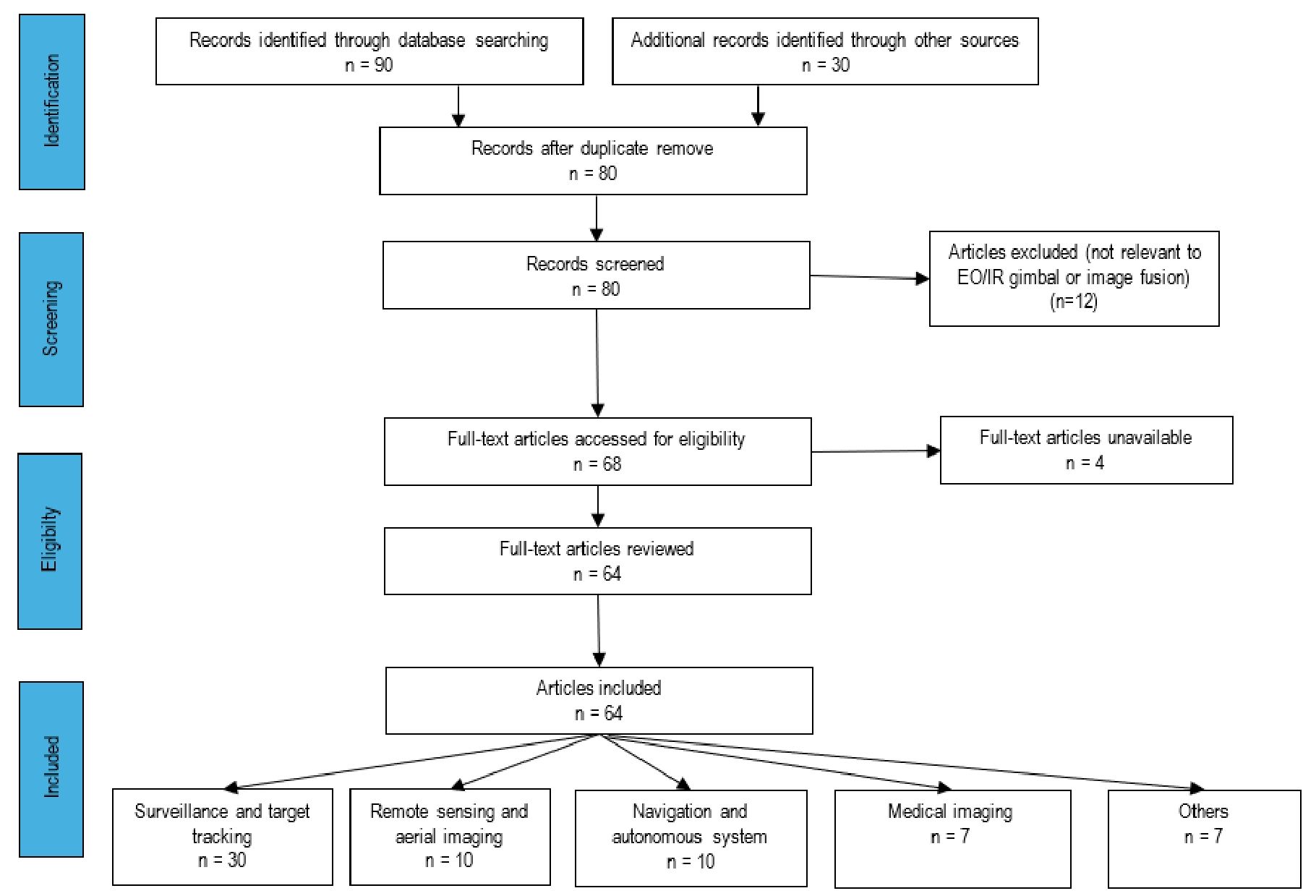
Fig. 1.
PRISMA flow diagram of this systematic review
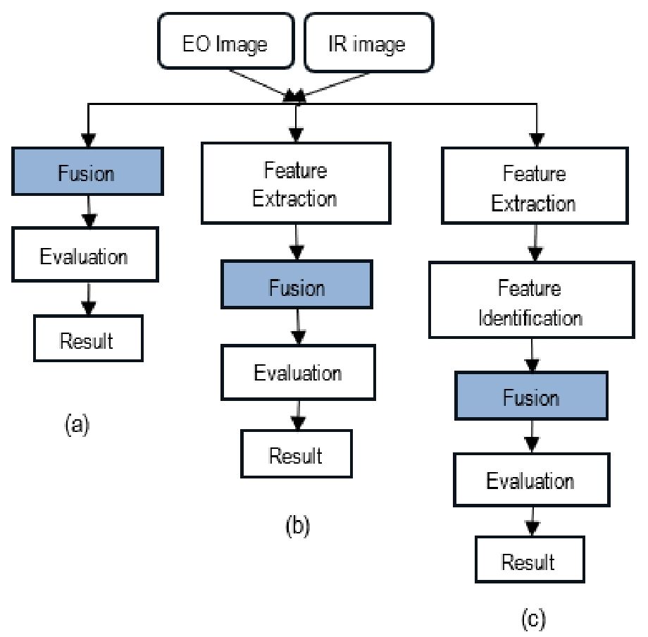
Fig. 2.
Image fusion framework a) pixel level b) feature level c) decision level
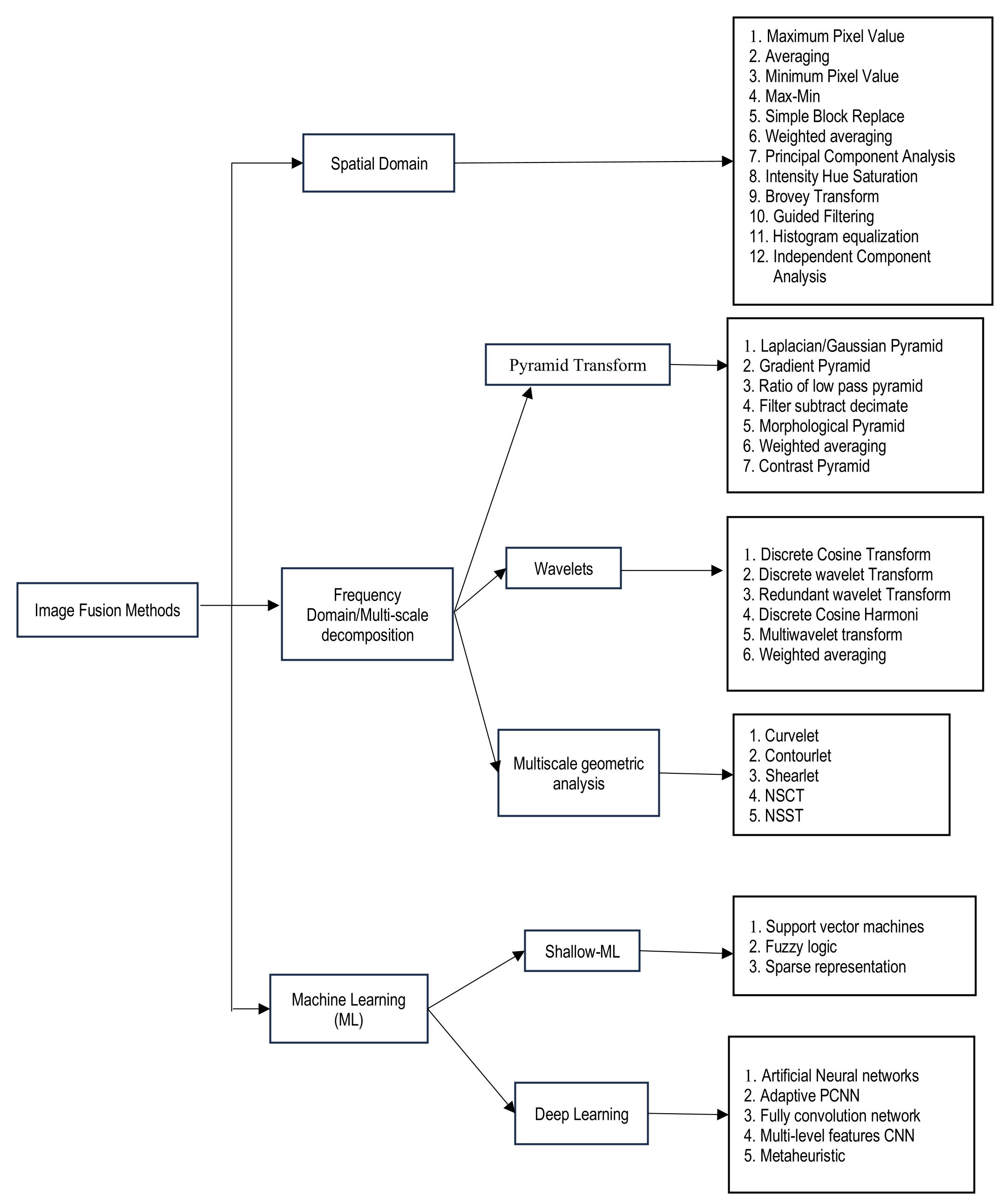
Fig. 3.
Image fusion techniques
Tab. 1.
Advantages and disadvantages of Spatial Domain Methods
| Fusion Method | Advantages | Disadvantages |
|---|---|---|
| Averaging - Image fusion by pixel averaging [22,23] | This is a basic method to identify and put into practice if the images are from the same sensor with lot of contrast and brightness. It involves a low computational cost | The fused image quality is reduced. The output images are hazy and so not suitable for real-time applications. Also, edges and image information are lost |
| Minimum pixel value [22] | The fused image is good if the inputs have dark shades | Fused images are characterised by low contrast and blurred |
| Simple block replacement [24] | Incredibly easy to understand and apply | The fused image has a random variation of brightness and color information. Fine detail of the image is less |
| Maximum pixel value [22,23] | The low pixel values are rejected, and the highest pixel value is used to create the fused method. So this method is susceptible to artifacts and distortion | The contrast of the fused image is decreased |
| Max-min [24] | Easy to implement, and the computational time is less | The efficiency of fusion is reduced, and the output image has rough edges due to blocking artifacts and isolated spots |
| Weighted averaging [25] | This method is easy to apply and robust. It is more suitable for multifocus images | The signal-to-noise ratio is enhanced in the fused image |
| PCA [26,27] | This approach gives excellent spatial quality and robust | Fused images show chromatic aberration and spectral degradation |
| IHS [23] | The colour, resolution and features are improved in the output image. The processing time is quick with high sharpening | Only three multispectral bands are analysed. So chromatic aberration occurs in the fused image |
| Brovey [24] | Extremely easy and fast processing method | RGB pictures are generated with high contrast, which causes color distortion |
| Guided filtering [28] | This method is suitable for real-time applications and provides better performance in image smoothing | The method does not apply to sparse input data. Some edges may have halos. Also, there will be a mismatch in the color and depth details between the input and fused image |
Tab. 2.
Advantages and Disadvantages of Frequency Domain Methods
| Fusion Method | Advantages | Disadvantages |
|---|---|---|
| Morphological pyramid [34] Laplacian/Gaussian pyramid [34,35] Gradient pyramid [36] Low-pass pyramid ratio [37] Filter subtract decimate [36] | Provide better image quality | The fused image is affected by the number of breakdown levels. Also, there is no direction information, so detailed image information in different directions cannot be extracted. |
| Discrete cosine transform (DCT) [38] | The images are decomposed into a series of cosine waveforms representing different spatial frequency components. This compact representation makes DCT suitable for real-time applications | The fused image is blurred, and blocking artifacts are generated. |
| Discrete wavelet technique with Haar fusion [39] | Spectral distortions are decreased, and a fused image with better SNR is produced. | The spatial resolution of the fused image is lower. The anisotropy of the source image is not represented. |
| Kekre’s wavelet transform fusion [40,41] | Irrespective of the size of the images, the fused image is more informative | Computation complexity is high |
| Kekre’s hybrid wavelet-based transform fusion [42,43] | Fused image results are better with more temporal and frequency features with multiresolution properties. | If the images are an integer power of two, this approach cannot be used |
| Stationary wavelet transform (SWT) [44-46] | At decomposition level 2, better results are obtained | High computational time |
| Curvelet Transform [47] | Best suits for edge representation | High computational time |
Tab. 3.
Advantages and Disadvantages of Deep Learning Methods
| Fusion Method | Advantages | Disadvantages |
|---|---|---|
| Convolution Neural Network [51-53] | Features are extracted and learnt from the training data without human assistance | Computational speed is low |
| CSR [54] | This method is less sensitive to misregistration | Enormous training data required |
| SAE [55] | Limited data required for supervised learning | The model training speed depends on the processor |
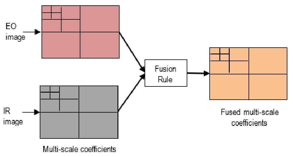
Fig. 4.
Generic structure of fusion rules
Tab. 4.
Performance Evaluation Metrics
| S. No. | Category | Metric | Desired value for good performance | Remarks |
|---|---|---|---|---|
| 1 | Information theory | Cross entropy (CE) | Low | Evaluates the similarity of information shared between the EO/IR image and the fused image |
| Entropy (EN) | High | Measures the average amount of information or detail contained in the fused image | ||
| Mutual information (MI) | High | Quantifies the degree of statistical dependence between the source and fused images. | ||
| Peak signal-to-noise ratio (PSNR) | High | Fused image distortion | ||
| 2 | Structural similarity | Universal image quality index, SSIM (Structural Similarity Index Metric) | High | Image loss (correlation loss, luminance loss) and distortion (contrast distortion) |
| Root Mean Squared Error (RMSE) | Low | Calculate the variation in the source image and the fused image | ||
| 3 | Image feature | Average gradient (AG) | High | Insights into image clarity and fusion texture characteristics |
| Edge intensity (EI) | High | Quantifies image edge intensity | ||
| Standard deviation (SD) | High | Provide details on the factors linked with image quality -distribution of information and contrast | ||
| Spatial frequency (SF) | High | Information on the overall activity and clarity of the image | ||
| Gradient-based fusion performance, QAB/F | High | Assesses the degree to which the gradient or edge details from the source images are preserved in the fused image |
Tab. 5.
| Data set | Algorithm | PSNR | SSIM | EN | MI | AG | SD | SF | Running time (s) |
|---|---|---|---|---|---|---|---|---|---|
| Multimodal image | Dense Fuse | 60.27 | 0.72 | 6.84 | 13.67 | 4.24 | - | - | 9.85 |
| CNN | 62.21 | 0.69 | 7.31 | 14.67 | 5.76 | - | - | 33.25 | |
| ResNet | 64.23 | 0.73 | 6.73 | 13.46 | 3.64 | - | - | 4.53 | |
| Convolution Sparse representation | - | 0.864 | 6.22 | 1.90 | - | 21.46 | - | - | |
| Anisotropic diffusion | - | 0.94 | 6.18 | 1.94 | - | 20.58 | - | - | |
| Fourth-order partial differential equation | - | 0.86 | 6.25 | 1.73 | - | 21.33 | - | - | |
| Total variation and augmented Lagrangian | - | 0.91 | 6.21 | 1.92 | - | 21.08 | - | - | |
| Bayes Fusion | - | 0.94 | 6.43 | 2.45 | - | 26.28 | - | - | |
| Deep convolutional sparse coding | - | - | 6.91 | 2.50 | 4.22 | 46.97 | - | - | |
| DeepFuse | - | - | 6.86 | 2.30 | 3.60 | 32.25 | - | - | |
| Saliency Detection | - | - | 6.67 | 1.72 | 3.98 | 28.04 | - | - | |
| FusianGAN | - | - | 6.58 | 2.34 | 2.42 | 29.04 | - | - | |
| DLF | - | - | 6.38 | 2.15 | 2.72 | 22.94 | - | - | |
| Fast and efficient zero learning | - | - | 6.63 | 2.23 | 2.55 | 28.09 | - | - | |
| Discrete Wavelet Transform (DWT) | - | - | 6.44 | - | 3.09 | - | 8.16 | 0.76 | |
| Non-subsampled contourlet transform (NSCT) | - | - | 7.17 | - | 5.02 | - | 12.78 | 2.03 | |
| Multi-Focus image fusion (MFCNN) | - | - | 6.61 | - | 3.61 | - | 9.55 | 0.38 | |
| CNN integration (ECNN) | - | - | 7.10 | - | 5.48 | - | 18.34 | 0.34 | |
| Unsupervised depth model for image fusion (SESF) | - | - | 7.31 | - | 7.26 | - | 24.91 | 0.31 | |
| IY-Net | - | - | 6.81 | - | 4.84 | - | 12.53 | 0.16 |