
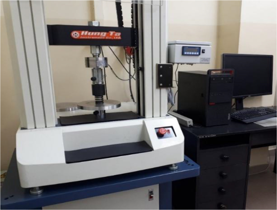
Fig. 1.
The testing machine used to spring axial stiffness researches
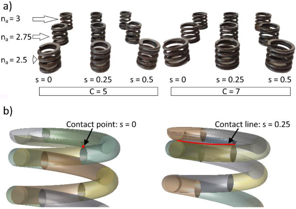
Fig. 2.
Samples of springs (a) used to axial stiffness researches; (b) graphical representation of contact length for two example lengths s = 0 and s = 0.25
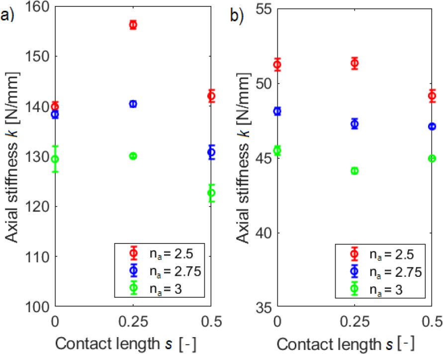
Fig. 3.
Axial stiffness k for different numbers of active coils na depending on the contact length per one side of spring s for a) C = 5, b) C = 7
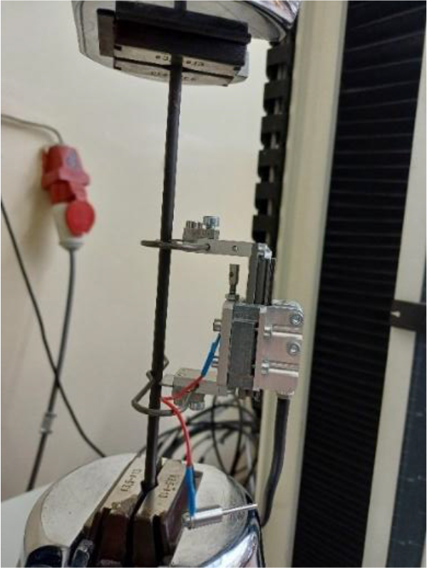
Fig. 4.
Young's modulus measurement station
Tab. 1.
Results of Young’s Modulus E measurement
| Wire number | Initial wire length L0 [mm] | Elongation L1 [mm] | Elongation L2 [mm] | Stress σ1 [MPa] | Stress σ2 [MPa] | Young's modulus [MPa] |
|---|---|---|---|---|---|---|
| 1 | 60.23 | 0.031 | 0.207 | 120 | 720 | 205330 |
| 2 | 60.82 | 0.031 | 0.211 | 120 | 720 | 202733 |
| Average Young's modulus E | 204031 | |||||
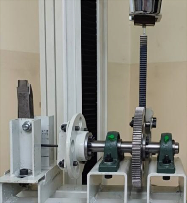
Fig. 5.
Kirchhoff's transverse elasticity modulus G measurement station
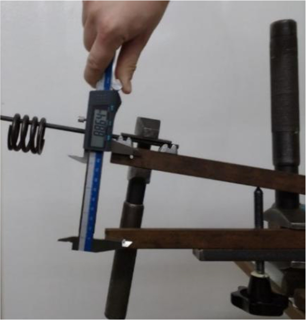
Fig. 6.
Measurement of the friction coefficient for steel-steel friction pair
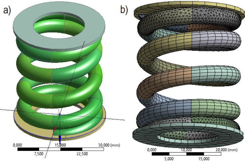
Fig. 7.
Spring with parameters C = 5, d = 5 mm, na = 2.5, s = 0.25 with supports a) modeled in the Design Modeler module of Ansys Workbench software, b) mesh used to stiffness calculation modeled in Static Structural module
Tab. 2.
Comparison of experimental data with numerical results.¥
| Spring index C | Active coils na | Contact length per ending s | Experimental stiffness k [N/mm] | FEM stiffness kFEM [N/mm] | Error [%] | Data range [%] | MAPE [%] |
|---|---|---|---|---|---|---|---|
| 5 | 2.5 | 0 | 140.8 | 143.6 | -2.0 | 8.7 | 3.6 |
| 0.25 | 155.9 | 148.5 | 6.7 | ||||
| 0.5 | 142.2 | 139.0 | 2.2 | ||||
| 3 | 0 | 128.0 | 121.4 | 5.1 | 2.2 | 3.7 | |
| 0.25 | 130.0 | 126.0 | 3.1 | ||||
| 0.5 | 121.2 | 117.7 | 2.9 | ||||
| 7 | 2.5 | 0 | 51.4 | 51.8 | -0.8 | 6.1 | 2.3 |
| 0.25 | 51.6 | 49.9 | 3.3 | ||||
| 0.5 | 49.5 | 50.9 | -2.8 | ||||
| 3 | 0 | 45.2 | 44.3 | 1.9 | 1.6 | 1.2 | |
| 0.25 | 43.9 | 43.8 | 0.4 | ||||
| 0.5 | 45.0 | 44.3 | 1.4 |
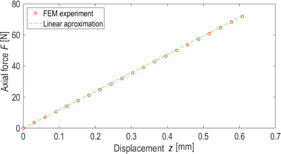
Fig. 8.
Force-displacement curve for a spring with C = 4, na = 1, γ = 10° for coil contact length s = 0.5
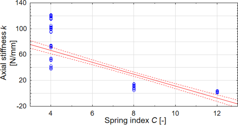
Fig. 9.
Correlation plot of axial stiffness k versus spring index C with coefficient r = -0.81
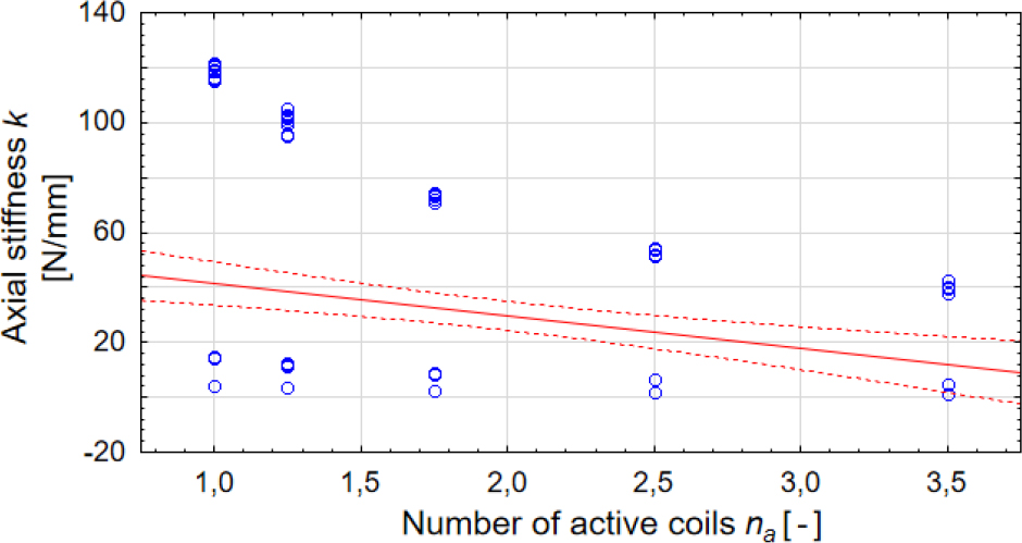
Fig. 10.
Correlation plot of axial stiffness k versus number of active coils na with coefficient r = -0.29
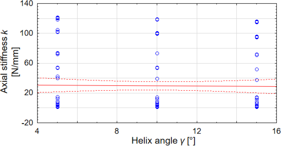
Fig. 11.
Correlation plot of axial stiffness k versus helix angle γ with coefficient r = -0.02
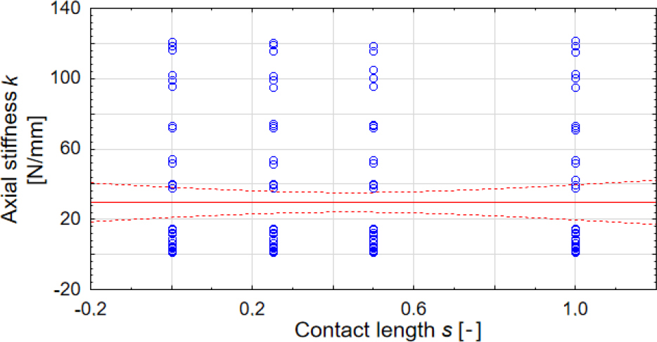
Fig. 12.
Correlation plot of axial stiffness k versus contact length per one ending s with coefficient r = -0.0002
Tab. 3.
Coefficient of variation of springs axial stiffness depending on spring angle, number of active coils and spring index
| Spring index C | Active coils na | Helix angle γ | ||
|---|---|---|---|---|
| 5° | 10° | 15° | ||
| 4 | 1 | 1.12% | 0.25% | 0.40% |
| 1.25 | 1.38% | 0.62% | 0.30% | |
| 1.75 | 1.17% | 0.30% | 0.59% | |
| 2.5 | 0.49% | 0.51% | 0.21% | |
| 3.5 | 2.82% | 0.20% | 0.12% | |
| 8 | 1 | 0.23% | 0.33% | 0.13% |
| 1.25 | 0.81% | 0.04% | 0.22% | |
| 1.75 | 0.64% | 0.36% | 0.31% | |
| 2.5 | 0.34% | 0.28% | 0.10% | |
| 3.5 | 0.14% | 0.13% | 0.17% | |
| 12 | 1 | 0.48% | 0.42% | 0.30% |
| 1.25 | 0.29% | 0.33% | 0.38% | |
| 1.75 | 0.35% | 0.17% | 0.92% | |
| 2.5 | 0.35% | 0.20% | 0.13% | |
| 3.5 | 0.13% | 0.22% | 0.22% | |
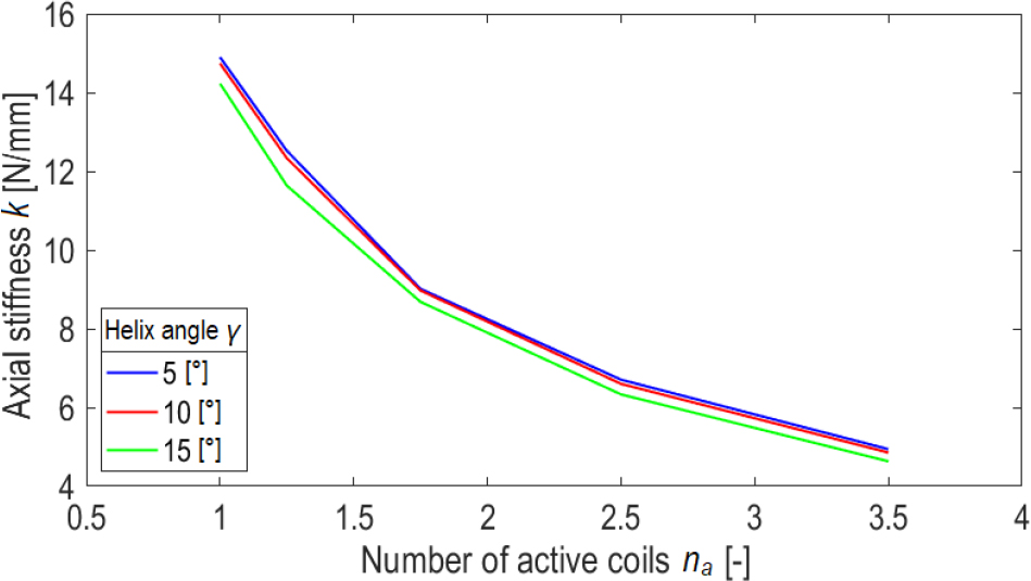
Fig. 13.
Axial stiffness for index C = 8, point contact (s = 0) for spring angles of 5, 10 and 15 degrees
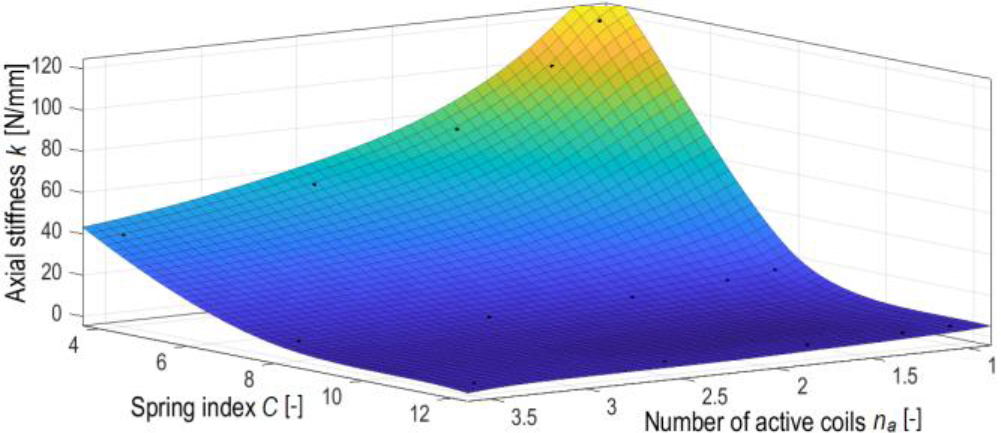
Fig. 14.
Axial stiffness distribution depending on the spring index C and the number of active coils na for the point contact of end coils
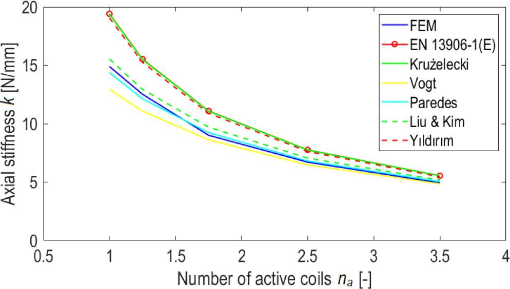
Fig. 15.
Axial stiffness k for the index C = 8, angle γ = 5°, point contact (s = 0) in comparison with selected analytical methods
Tab. 4.
The values of coefficient a and b of equation (13) depending on the spring index C and helix angle γ together with the given R-square parameter
| C | γ [°] | a | b | R2 |
|---|---|---|---|---|
| 4 | 5 | 4.550 | 0.6462 | 0.8685 |
| 10 | 4.328 | 0.5942 | 0.9889 | |
| 15 | 3.946 | 0.4576 | 0.9917 | |
| 8 | 5 | 4.409 | 0.5350 | 0.9164 |
| 10 | 4.168 | 0.4938 | 0.9726 | |
| 15 | 3.701 | 0.3970 | 0.9961 | |
| 12 | 5 | 4.393 | 0.5183 | 0.9021 |
| 10 | 4.055 | 0.4600 | 0.9751 | |
| 15 | 3.587 | 0.3937 | 0.9910 |
Tab. 5.
The values of coefficient k1 k2, m1, m2 of equations (14) and (15) depending on the spring index with the given R-square parameter
| C | k1 | k2 | R2 | m1 | m2 | R2 |
|---|---|---|---|---|---|---|
| 4 | -0.060 | 4.879 | 0.9771 | -0.019 | 0.755 | 0.9371 |
| 8 | -0.071 | 4.801 | 0.9672 | -0.014 | 0.613 | 0.9487 |
| 12 | -0.081 | 4.818 | 0.9914 | -0.012 | 0.582 | 0.9986 |
| Av. | -0.071 | 4.833 | 0.9786 | -0.015 | 0.650 | 0.9615 |
Tab. 6.
Comparison of parameters a and b calculated using equations (16) and (17) with the target values
| C | γ [°] | a | a (16) | b | b (17) |
|---|---|---|---|---|---|
| 4 | 5 | 4.550 | 4.478 | 0.6462 | 0.575 |
| 10 | 4.328 | 4.123 | 0.5942 | 0.5 | |
| 15 | 3.946 | 3.768 | 0.4576 | 0.425 | |
| 8 | 5 | 4.409 | 4.478 | 0.5350 | 0.575 |
| 10 | 4.168 | 4.123 | 0.4938 | 0.5 | |
| 15 | 3.701 | 3.768 | 0.3970 | 0.425 | |
| 12 | 5 | 4.393 | 4.478 | 0.5183 | 0.575 |
| 10 | 4.055 | 4.123 | 0.4600 | 0.5 | |
| 15 | 3.587 | 3.768 | 0.3937 | 0.425 | |
| R2 | 0.9786 | R2 | 0.9615 | ||
Tab. 7.
Comparison of the accuracy of selected methods for calculating the axial stiffness of compression springs
| Axial stiffness formula | Mean absolute percentage error (MAPE) |
|---|---|
| EN 13906-1:2013(E) norm (1) | 23.40% |
| Vogt (1934) (2) | 5.91% |
| Paredes (2016) (2) | 3.62% |
| Krużelecki and Życzkowski (1990) (3) | 22.17% |
| Yıldırım (2016) (4) | 18.95% |
| Liu and Kim (2009) (5) | 13.93% |
| kχ (18) | 1.38% |
Tab. 8.
Comparison of axial stiffness values calculated using the most accurate methods and the commonly used Eq. (1) with bench test results
| Spring index C | Active coils na | Contacting coils per ending s | Experimental mean stiffness [N/mm] | kN (1) | kχ (18) | kP (2) |
|---|---|---|---|---|---|---|
| Error to experimental value [%] | ||||||
| 5 | 2.5 | 0 | 139.9 | -15 | 1 | -1 |
| 0.25 | 156.3 | -3 | 12 | 10 | ||
| 0.5 | 142.0 | -13 | 3 | 1 | ||
| 2.75 | 0 | 138.4 | -6 | 8 | 6 | |
| 0.25 | 140.5 | -4 | 10 | 7 | ||
| 0.5 | 130.8 | -12 | 3 | 1 | ||
| 3 | 0 | 129.4 | -4 | 10 | 7 | |
| 0.25 | 130.0 | -3 | 10 | 8 | ||
| 0.5 | 122.7 | -9 | 5 | 2 | ||
| MAPE [%] | 8 | 7 | 5 | |||
| Gap [%] | 12 | 10 | 11 | |||
| 7 | 2.5 | 0 | 51.2 | -15 | 1 | -1 |
| 0.25 | 51.3 | -14 | 1 | 0 | ||
| 0.5 | 49.2 | -19 | -4 | -5 | ||
| 2.75 | 0 | 48.1 | -11 | 3 | 2 | |
| 0.25 | 47.3 | -13 | 1 | 0 | ||
| 0.5 | 47.1 | -13 | 1 | -1 | ||
| 3 | 0 | 45.5 | -8 | 5 | 4 | |
| 0.25 | 44.1 | -11 | 2 | 1 | ||
| 0.5 | 45.0 | -9 | 4 | 3 | ||
| MAPE [%] | 13 | 2 | 2 | |||
| Gap [%] | 12 | 9 | 8 | |||
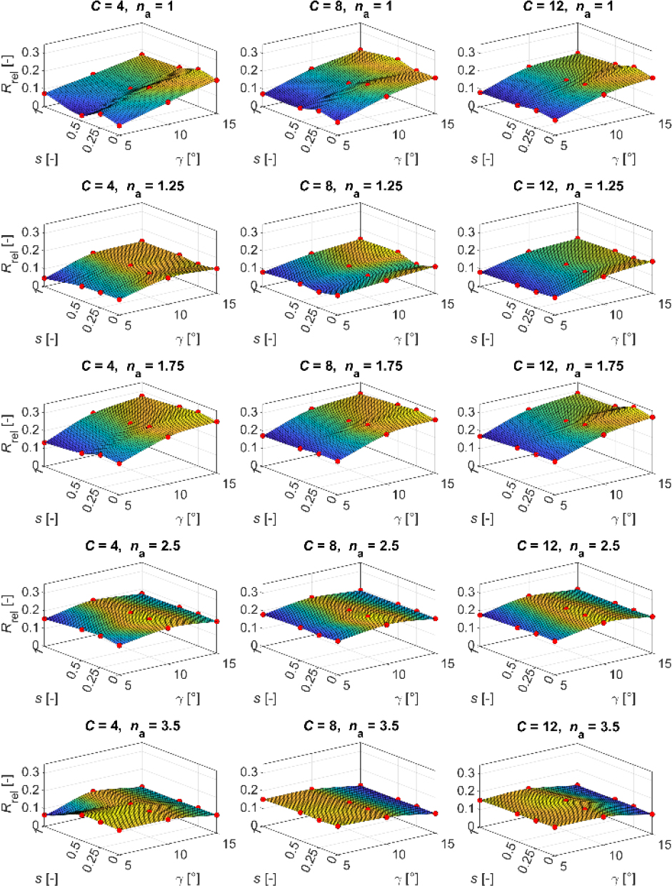
Fig. 16.
Plots of the Rrel dependency on the contact length and the helix pitch angle for springs with a given spring index C and number of active coils na
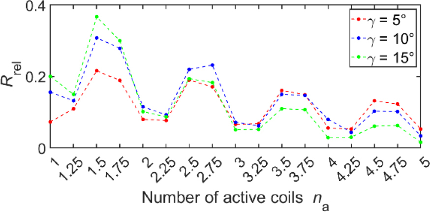
Fig. 17.
Plots of the Rrel dependency on the number of active coils na for helix pitch angles γ: 5°, 10°, 15°, for springs with C = 8 oraz s = 0
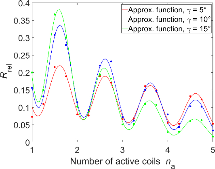
Fig. 18.
Preliminary approximation plots of Rrel as a function of the number of active coils na for helix pitch angles of 5° 10° and 15°, for springs with C = s and = 0
Tab. 9.
The values of the function coefficients Eq. (20), along with the coefficients of determination
| γ [°] | c1 | c2 | c3 | c4 | R-square |
|---|---|---|---|---|---|
| 5 | 0.0685 | -0.1508 | 2.7048 | 1.2563 | 0.9862 |
| 10 | 0.1660 | -0.3381 | 2.1928 | 0.8522 | 0.9853 |
| 15 | 0.2731 | -0.5805 | 2.1819 | 0.9409 | 0.9948 |
Tab. 10.
The approximation results with fixed values of coefficients
| γ [°] | c1 | c2 | c3 | c4 | R-square |
|---|---|---|---|---|---|
| 5 | 0.0787 | -0.1529 | 2.3598 | 1.0165 | 0.9760 |
| 10 | 0.1541 | -0.3385 | 0.9796 | ||
| 15 | 0.2502 | -0.5745 | 0.9934 |
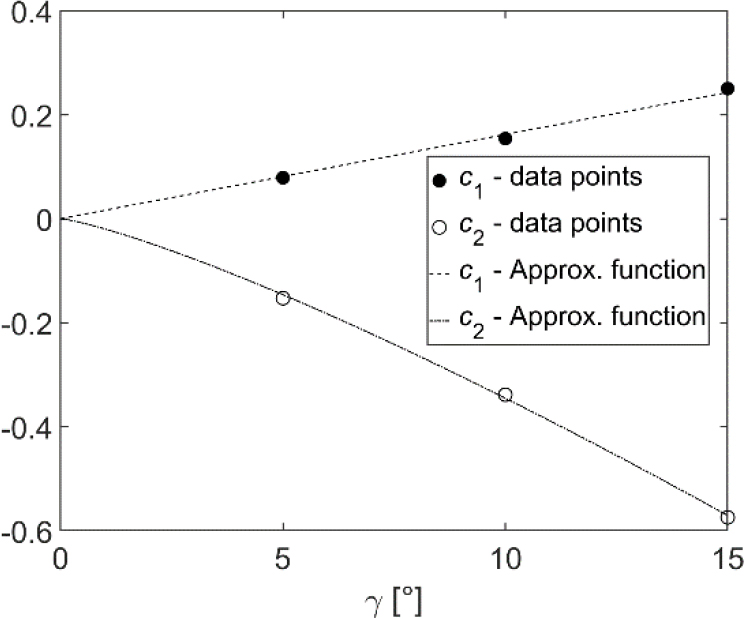
Fig. 19.
Approximation plots of coefficients c1 and c2 along with the data for springs with C = s and = 0
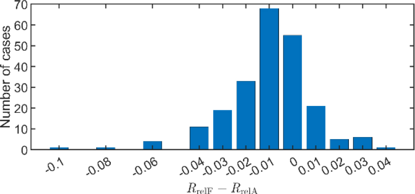
Fig. 20.
Distribution of the number of particular cases with specific values of difference RrelF — RrelA
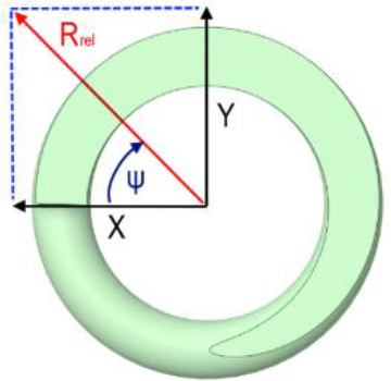
Fig. 21.
The coordinate system used to determine the transverse reaction angle Rrel. Top view of the spring
Tab. 11.
Results of the transverse reaction angle ψ test due to axial compression – basic 225 results
| Active coils na | Contact length s | Angle of reaction ψ [°] | Active coils na | Contact length s | Angle of reaction ψ [°] |
|---|---|---|---|---|---|
| 1 | 0 | 90 | 2.25 | 0 | 315 |
| 1 | 0.25 | 180 | 2.5 | 0 | 0 |
| 1 | 0.5 | 270 | 2.5 | 0.25 | 90 |
| 1 | 1 | 90 | 2.5 | 0.5 | 180 |
| 1.25 | 0 | 315 | 2.5 | 1 | 0 |
| 1.25 | 0.25 | 45 | 2.75 | 0 | 45 |
| 1.25 | 0.5 | 135 | 3 | 0 | 90 |
| 1.25 | 1 | 315 | 3.25 | 0 | 315 |
| 1.5 | 0 | 0 | 3.5 | 0 | 0 |
| 1.5 | 0.25 | 90 | 3.5 | 0.25 | 90 |
| 1.5 | 0.5 | 180 | 3.5 | 0.5 | 180 |
| 1.5 | 1 | 0 | 3.5 | 1 | 0 |
| 1.75 | 0 | 45 | 3.75 | 0 | 45 |
| 1.75 | 0.25 | 135 | 4 | 0 | 90 |
| 1.75 | 0.5 | 225 | 4.25 | 0 | 315 |
| 1.75 | 1 | 45 | 4.5 | 0 | 0 |
| 2 | 0 | 90 | 4.75 | 0 | 45 |
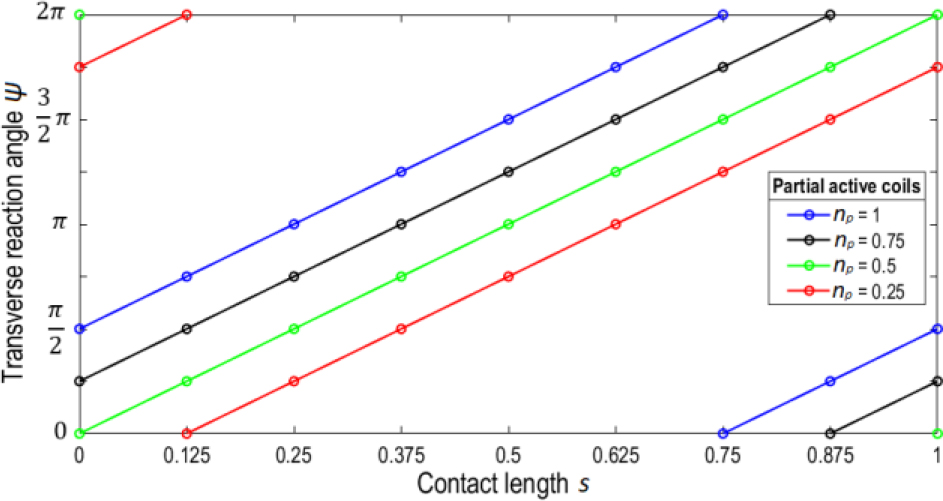
Fig. 22.
Graph of functions describing the dependence of the transverse reaction angle ψ on the contact length s and the partial number of active coils np