
FIGURE 1.
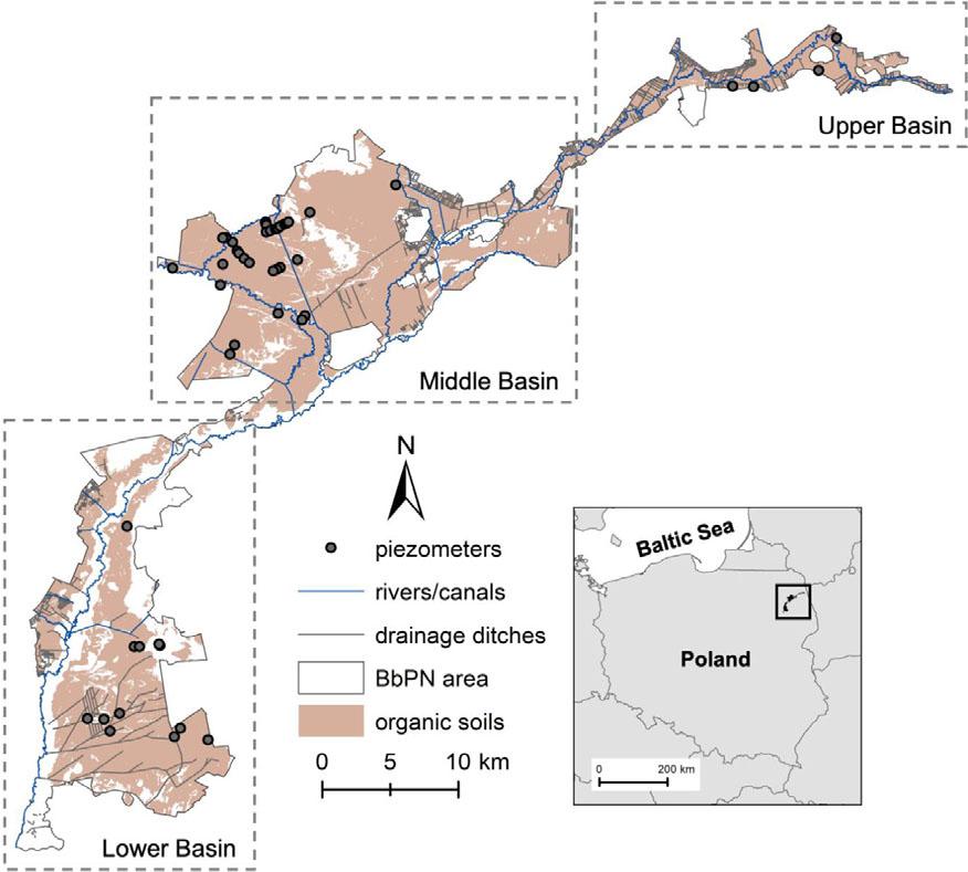
FIGURE 2.
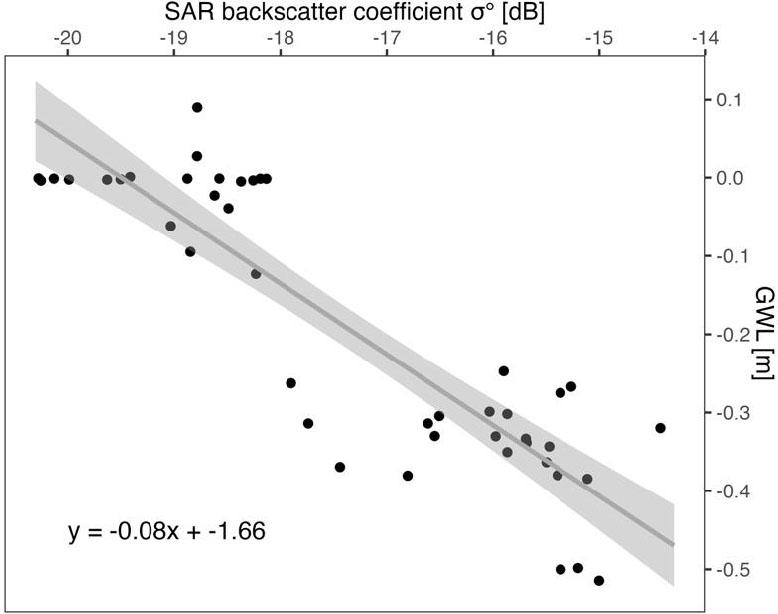
FIGURE 3.

FIGURE 4.
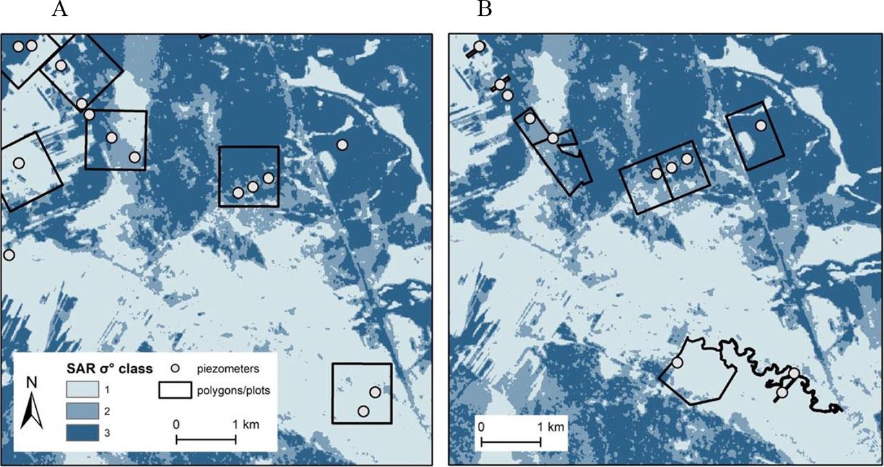
FIGURE 5.
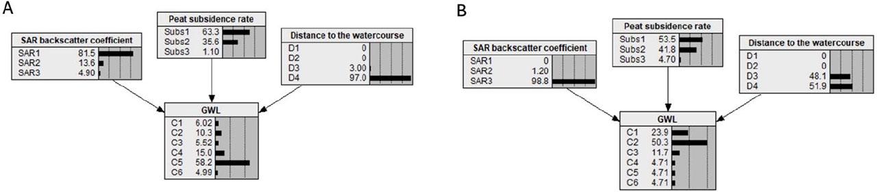
FIGURE 6.
Classification of parameters used in the Bayesian network modela
| Parameter | Class | Value |
|---|---|---|
| Groundwater level [m] | C1 | < −0.4 |
| C2 | −0.4 to −0.3 | |
| C3 | −0.3 to −0.2 | |
| C4 | −0.2 to −0.1 | |
| C5 | −0.1 to 0.0 | |
| C6 | > 0.0 | |
| SAR backscatter coefficient (σ°) [dB] | SAR1 | < −18 |
| SAR2 | −18 to −16 | |
| SAR3 | > −16 | |
| Peat subsidence rate [m·year−1] | Subs1 | −0.05 to −0.02 |
| Subs2 | −0.02 to −0.01 | |
| Subs3 | −0.01 to 0.05 | |
| Distance to the watercourse [m] | D1 | 0 to 25 |
| D2 | 25 to 100 | |
| D3 | 100 to 440 | |
| D4 | > 440 |
Spearman’s rank correlation results between model variables
| Pair of compared model variables | Spearman’s rank correlation parameters | |
|---|---|---|
| ρ | p-value | |
| Synthetic aperture radar backscatter coefficient–subsidence | −0.11 | 0.47 |
| Synthetic aperture radar backscatter coefficient–distance to the watercourses | 0.11 | 0.45 |
| Subsidence–distance to the watercourses | −0.03 | 0.82 |
Piezometers within the Biebrza National Park used in the study
| ID | Piezometer/Transect name | Start of measurement | End of measurement | Mean GWT [m] |
|---|---|---|---|---|
| 1 | – | 2014 | 2022 | 0.001 |
| 2 | – | 2015 | 2022 | −0.002 |
| 3 | – | 2014 | 2021 | −0.004 |
| 4 | – | 2014 | 2021 | −0.004 |
| 5 | – | 2015 | 2021 | −0.003 |
| 6 | – | 2015 | 2021 | −0.001 |
| 7 | – | 2015 | 2021 | −0.004 |
| 8 | – | 2014 | 2021 | −0.002 |
| 9 | – | 2015 | 2021 | −0.001 |
| 10 | – | 2015 | 2021 | −0.001 |
| 11 | – | 2017 | 2021 | −0.001 |
| 12 | – | 2015 | 2021 | −0.001 |
| 13 | – | 2011 | 2018 | −0.001 |
| 14 | Brzeziny Ciszewskie | 1998 | 2022 | −0.343 |
| 15 | Brzeziny Ciszewskie | 1998 | 2022 | −0.320 |
| 16 | Ciszewo | 1994 | 2022 | −0.351 |
| 17 | Ciszewo | 1994 | 2022 | −0.267 |
| 18 | Ciszewo | 1994 | 2022 | −0.380 |
| 19 | Ciszewo | 1994 | 2022 | −0.247 |
| 20 | Ciszewo | 1994 | 2022 | −0.314 |
| 21 | Czerwone Bagno T | 2008 | 2015 | −0.062 |
| 22 | Czerwone Bagno T | 2008 | 2015 | −0.039 |
| 23 | Długa Luka | 2009 | 2022 | −0.023 |
| 24 | Grobla Honczarowska | 1998 | 2022 | 0.027 |
| 25 | Grobla Honczarowska | 1998 | 2022 | 0.089 |
| 26 | Grobla Honczarowska | 1998 | 2022 | −0.010 |
| 27 | Grzędy I | 1996 | 2022 | −0.385 |
| 28 | Grzędy I | 1996 | 2022 | −0.498 |
| 29 | Grzędy I | 1996 | 2022 | −0.363 |
| 30 | Grzędy I | 1996 | 2022 | −0.381 |
| 31 | Grzędy I | 1996 | 2022 | −0.330 |
| 32 | Grzędy II | 1996 | 2022 | −0.514 |
| 33 | Gugny | 2009 | 2022 | −0.123 |
| 34 | Gugny | 2009 | 2022 | −0.095 |
| 35 | Gugny II | 2009 | 2022 | −0.085 |
| 36 | Gugny II | 2009 | 2022 | −0.125 |
| 37 | Gugny II | 2009 | 2022 | −0.012 |
| 38 | Jałowo | 1998 | 2022 | −0.302 |
| 39 | Jałowo | 1998 | 2022 | −0.034 |
| 40 | Kapice | 2012 | 2021 | −0.263 |
| 41 | Kuligi | 1994 | 2022 | −0.314 |
| 42 | Kuligi | 1994 | 2022 | −0.330 |
| 43 | Kuligi | 1994 | 2022 | −0.369 |
| 44 | Trójkąt I | 1996 | 2022 | −0.333 |
| 45 | Trójkąt I | 1996 | 2022 | −0.338 |
| 46 | Trójkąt I | 1996 | 2022 | −0.500 |
| 47 | Trójkąt II | 1996 | 2022 | −0.275 |
| 48 | Trójkąt II | 1996 | 2022 | −0.299 |
| 49 | Trójkąt II | 1996 | 2022 | −0.304 |
Conditional probabilities of groundwater level classes generated from the Bayesian belief network
| V.m. | No | Avg. obs. GWL [m] | GWL class probability [%] | GWL class | ||||||
|---|---|---|---|---|---|---|---|---|---|---|
| C1 | C2 | C3 | C4 | C5 | C6 | Obs. | Pred. | |||
| Polygon | 1 | −0.364 | 10 | 28.5 | 10.6 | 6.95 | 37.8 | 6.05 | C2 | C5 |
| 2 | −0.293 | 5.96 | 22.5 | 52 | 5.83 | 7.85 | 5.82 | C3 | C3 | |
| 3 | −0.391 | 20.8 | 50.8 | 7.07 | 5.87 | 9.66 | 5.79 | C2 | C2 | |
| 4 | −0.314 | 7.38 | 39.1 | 14 | 6.76 | 27 | 5.73 | C2 | C2 | |
| 5 | −0.309 | 10.6 | 34.4 | 20.8 | 6.52 | 21.4 | 6.19 | C2 | C2 | |
| 6 | −0.332 | 16.9 | 35.4 | 9.91 | 7.63 | 23.4 | 6.77 | C2 | C2 | |
| 7 | −0.001 | 6.94 | 8.55 | 7.25 | 6.94 | 59.7 | 10.6 | C5 | C5 | |
| 8 | −0.006 | 8.67 | 12.6 | 9.17 | 7.98 | 48.8 | 12.8 | C5 | C5 | |
| 9 | −0.004 | 6.02 | 10.3 | 5.52 | 15 | 58.2 | 4.99 | C5 | C5 | |
| 10 | −0.002 | 7.03 | 29.1 | 10.5 | 8.04 | 38.8 | 6.51 | C5 | C5 | |
| 11 | −0.109 | 6.17 | 13.5 | 8.09 | 7.99 | 59.4 | 4.89 | C4 | C5 | |
| 12 | −0.012 | 5.74 | 7.16 | 5.88 | 8.61 | 65.6 | 6.98 | C5 | C5 | |
| BbPN plot | 1 | −0.002 | 6.68 | 21 | 8.24 | 8.87 | 49.5 | 5.71 | C5 | C5 |
| 2 | −0.338 | 7.9 | 50.4 | 9.52 | 6.23 | 19.9 | 6.05 | C2 | C2 | |
| 3 | −0.500 | 14.2 | 34.2 | 16.6 | 9.9 | 14.7 | 10.4 | C1 | C2 | |
| 4 | −0.338 | 5.26 | 67.8 | 10.4 | 5.26 | 6.08 | 5.26 | C2 | C2 | |
| 5 | −0.351 | 20.6 | 56.2 | 4.64 | 4.64 | 9.24 | 4.64 | C2 | C2 | |
| 6 | −0.267 | 4.57 | 52.3 | 18.6 | 4.57 | 15.4 | 4.57 | C3 | C2 | |
| 7 | 0.001 | 7.75 | 7.75 | 7.75 | 7.75 | 55.2 | 14.2 | C6 | C5 | |
| 8 | −0.002 | 6.06 | 6.06 | 6.06 | 6.06 | 67.8 | 7.93 | C5 | C5 | |
| 9 | −0.304 | 6.49 | 30.2 | 32.1 | 6.44 | 18.4 | 6.4 | C2 | C3 | |
| 10 | −0.001 | 10.2 | 38.7 | 10.5 | 7.78 | 25.3 | 7.45 | C5 | C2 | |
| 11 | −0.003 | 5.72 | 15.6 | 8.9 | 7.11 | 57 | 5.72 | C5 | C5 | |
| 12 | −0.287 | 6.65 | 16.9 | 52.8 | 6.65 | 10.4 | 6.65 | C3 | C3 | |
| 13 | −0.314 | 9.32 | 49.5 | 20.8 | 6.24 | 7.95 | 6.14 | C2 | C2 | |
| 14 | −0.514 | 19.6 | 44.7 | 9.63 | 6.48 | 13.4 | 6.13 | C1 | C2 | |
| 15 | −0.247 | 6.51 | 56 | 18.9 | 6.03 | 6.52 | 6.02 | C3 | C2 | |
| 16 | −0.333 | 8.04 | 35.7 | 26.6 | 5.77 | 18.4 | 5.45 | C2 | C2 | |
| 17 | −0.372 | 21.7 | 52.8 | 6.65 | 5.35 | 8.17 | 5.3 | C2 | C2 | |
| 18 | −0.062 | 9.27 | 24.3 | 12.8 | 7.14 | 39 | 7.47 | C5 | C5 | |
| 19 | −0.005 | 6.14 | 11.8 | 6.24 | 7.86 | 61.6 | 6.37 | C5 | C5 | |
| 20 | −0.023 | 6.51 | 6.51 | 6.51 | 6.51 | 66.4 | 7.54 | C5 | C5 | |
| 21 | −0.001 | 5.81 | 8.9 | 5.78 | 10.9 | 63 | 5.61 | C5 | C5 | |
| 22 | −0.001 | 3.93 | 3.93 | 3.93 | 3.93 | 74.6 | 3.93 | C5 | C5 | |
| 23 | −0.001 | 8.24 | 10.6 | 9.72 | 8.08 | 47.8 | 15.6 | C5 | C5 | |
| 24 | −0.001 | 11.8 | 17.5 | 11.7 | 9.62 | 36.4 | 12.9 | C5 | C5 | |
| 25 | −0.001 | 12.1 | 22 | 11.5 | 9.08 | 33.5 | 11.9 | C5 | C5 | |
| 26 | −0.320 | 23.9 | 50.3 | 11.7 | 4.71 | 4.71 | 4.71 | C2 | C2 | |
Area percentage contributions of each model variables class in polygons and plots used for validation
| V.m. | No | Area [ha] | Avg. obs. GWL [m] | SAR backscatter coefficient class distribution [%] | Subsidence class distribution [%] | Distance to the watercourse class distribution [%] | |||||||
|---|---|---|---|---|---|---|---|---|---|---|---|---|---|
| 1 | 2 | 3 | 1 | 2 | 3 | 1 | 2 | 3 | 4 | ||||
| Polygon | 1 | 100 | −0.364 | 48.3 | 21.9 | 29.8 | 21.7 | 60 | 18.3 | 0 | 4 | 53.4 | 42.6 |
| 2 | 100 | −0.293 | 3.5 | 26.7 | 69.8 | 0.6 | 31.4 | 68 | 0 | 0 | 0 | 100 | |
| 3 | 100 | −0.391 | 6.6 | 11.9 | 81.5 | 64.3 | 34.6 | 1.1 | 3.6 | 10.4 | 71.6 | 14.4 | |
| 4 | 100 | −0.314 | 30.1 | 41.0 | 28.9 | 17.1 | 76 | 6.9 | 0 | 0 | 0 | 100 | |
| 5 | 100 | −0.309 | 23.2 | 22.8 | 54.0 | 11.1 | 57.2 | 31.7 | 0 | 0.7 | 35.3 | 64 | |
| 6 | 100 | −0.332 | 29.6 | 4.4 | 66.0 | 52.9 | 44.8 | 2.3 | 5.8 | 13.5 | 40.4 | 40.3 | |
| 7 | 100 | −0.001 | 96.0 | 4.0 | 0.0 | 24.3 | 65.6 | 10.1 | 10.6 | 23.4 | 66 | 0 | |
| 8 | 100 | −0.006 | 79.9 | 10.3 | 9.8 | 11 | 55.9 | 33.1 | 15.5 | 41.2 | 43.3 | 0 | |
| 9 | 100 | −0.004 | 81.5 | 13.6 | 4.9 | 63.3 | 35.6 | 1.1 | 0 | 0 | 3 | 97 | |
| 10 | 100 | −0.002 | 48.6 | 46,0 | 5.4 | 22.6 | 60.5 | 16.9 | 0.3 | 1.7 | 25.9 | 72.1 | |
| 11 | 100 | −0.109 | 79.8 | 6.6 | 13.6 | 22.6 | 65.2 | 12.2 | 0 | 0 | 14.1 | 85.9 | |
| 12 | 100 | −0.012 | 96.7 | 3.3 | 0.0 | 34.6 | 61.5 | 3.9 | 4 | 10.8 | 42.4 | 42.8 | |
| BbPN plot | 1 | 5.72 | −0.002 | 64.6 | 27.4 | 8 | 30 | 60 | 10 | 0 | 0 | 18.5 | 81.5 |
| 2 | 4.75 | −0.338 | 20.3 | 65.8 | 13.9 | 10 | 80 | 10 | 0 | 1.3 | 53.9 | 44.8 | |
| 3 | 1.41 | −0.5 | 10.7 | 44.3 | 45 | 33.3 | 66.7 | 0 | 13.6 | 45.5 | 40.9 | 0 | |
| 4 | 0.92 | −0.338 | 1.1 | 78.4 | 20.5 | 0 | 100 | 0 | 0 | 0 | 0 | 100 | |
| 5 | 1.74 | −0.351 | 6.9 | 24.7 | 68.4 | 33.3 | 66.7 | 0 | 0 | 0 | 100 | 0 | |
| 6 | 1.73 | −0.267 | 14.4 | 29.3 | 56.3 | 0 | 100 | 0 | 0 | 0 | 0 | 100 | |
| 7 | 7.21 | 0.001 | 100 | 0 | 0 | 33.3 | 41.7 | 25 | 22.5 | 25 | 52.5 | 0 | |
| 8 | 1.3 | −0.002 | 100 | 0 | 0 | 0 | 33.3 | 66.7 | 4.8 | 19 | 76.2 | 0 | |
| 9 | 53.24 | −0.304 | 19.3 | 56.1 | 24.6 | 1.1 | 47.8 | 51.1 | 0 | 0 | 0 | 100 | |
| 10 | 38.63 | −0.001 | 29.2 | 50.7 | 20.1 | 32.8 | 61.2 | 6 | 3.3 | 10.2 | 52.6 | 33.9 | |
| 11 | 18.46 | −0.003 | 76.7 | 23.3 | 0 | 9.1 | 63.6 | 27.3 | 0 | 0 | 0 | 100 | |
| 12 | 53.57 | −0.287 | 6.8 | 47.8 | 45.4 | 0 | 18.7 | 81.3 | 0 | 0 | 0 | 100 | |
| 13 | 50.47 | −0.314 | 2.6 | 46.9 | 50.5 | 18.9 | 71.1 | 10 | 0 | 0 | 0 | 100 | |
| 14 | 65.53 | −0.514 | 12.3 | 9.9 | 77.8 | 53.8 | 43.4 | 2.8 | 3.6 | 9.8 | 52.8 | 33.8 | |
| 15 | 19.53 | −0.247 | 0.7 | 73.6 | 25.7 | 5.7 | 80 | 14.3 | 0 | 0 | 0 | 100 | |
| 16 | 50.94 | −0.333 | 19.4 | 20.3 | 60.3 | 9 | 64 | 27 | 0 | 0 | 8.8 | 91.2 | |
| 17 | 39.29 | −0.372 | 4.7 | 10 | 85.3 | 57.1 | 42.9 | 0 | 2.1 | 8.9 | 76.1 | 12.9 | |
| 18 | 61.39 | −0.062 | 50.6 | 22.4 | 27 | 4.6 | 55 | 40.4 | 2.4 | 8.9 | 54.4 | 34.3 | |
| 19 | 87.01 | −0.005 | 87 | 10.1 | 2.9 | 31 | 65.2 | 3.8 | 2.3 | 7.5 | 50 | 40.2 | |
| 20 | 2.01 | −0.023 | 100 | 0 | 0 | 33.3 | 66.7 | 0 | 3.1 | 15.6 | 81.3 | 0 | |
| 21 | 450.55 | −0.001 | 90.3 | 5.2 | 4.5 | 44.3 | 51.1 | 4.6 | 2 | 4.8 | 21.4 | 71.8 | |
| 22 | 3.86 | −0.001 | 100 | 0 | 0 | 28.6 | 71.4 | 0 | 0 | 0 | 0 | 100 | |
| 23 | 41.17 | −0.001 | 86.5 | 10.7 | 2.8 | 13.7 | 64.4 | 21.9 | 21.9 | 47.7 | 30.4 | 0 | |
| 24 | 2.19 | −0.001 | 50.9 | 12.7 | 36.4 | 0 | 66.7 | 33.3 | 14.7 | 50 | 35.3 | 0 | |
| 25 | 1.78 | −0.001 | 44.3 | 19.9 | 35.8 | 0 | 66.7 | 33.3 | 14.3 | 35.7 | 50 | 0 | |
| 26 | 24.2 | −0.320 | 0 | 1.2 | 98.8 | 53.5 | 41.8 | 4.7 | 0 | 0 | 48.1 | 51.9 | |