
Contemporary management of peatlands requires documentation of their current state to serve as a baseline for future evaluations within an adaptive management approach (United Nations Environment Programme [UNEP], 2022). One critical aspect of this documentation is assessing greenhouse gas (GHG) fluxes. There is a pressing global demand for accurate estimates of GHG emissions from peatlands to inform management strategies and enhance decision-making processes. This need is underscored by the challenges associated with implementing policies such as the recently enacted EU Nature Restoration Law ( European Commission [EC], 2022), which calls for measures that incentivize farmers to mitigate GHG emissions from drained peatlands by raising groundwater levels (GWL) on their lands (Liu et al., 2023). Rewetting is usually the first step in the restoration process of peatlands (Grand-Clement et al., 2015), as all the other elements and functions are dependent on the presence of water (Jones et al., 2018). Accurate GHG emission data is crucial for providing indicators of the effectiveness of rewetting activities (Nielsen et al., 2023). This is especially important for determining appropriate subsidies based on the activities undertaken by farmers. However, direct measurement of GHG fluxes is often unfeasible due to the high costs, time, and specialized personnel required (Cieśliński, 2024). As a result, there is a growing demand for alternative, simplified methods of estimating GHG emissions from drained peatlands.
Peatlands’ GWL is recognized as the most informative proxy for GHG emissions (Tanneberger et al., 2024). It was found to be the most sensitive and influential factor affecting gas fluxes, with even minor changes in GWL (on the order of centimeters) capable of causing significant variations in carbon dioxide emissions (Tiemeyer et al., 2020; Evans et al., 2021; Koch et al., 2023). Yet, measuring the GWL also requires field inspections, and obtaining multi-year average GWL data to assess the status or pre- and post-rewetting differences is equally costly, time-consuming (Ghazaryan et al., 2024) and requires meticulous planning of the location of monitoring wells. Therefore, developing a method for predicting the GWL in peatlands using readily available, long-term datasets, such as those derived from remote sensing, is essential.
Various remote sensing data types and sources are widely used in peatland monitoring (Harris & Bryant, 2009; Lees et al., 2018; Millard et al., 2018; Food and Agriculture Organization of the United Nations [FAO], 2021; Habib & Connolly, 2023; Ghezelayagh et al., 2024). However, no universally applicable and accurate tool or methodology has been implemented to assess GWL in peatlands globally. The choice of remote sensing datasets depends on the specific parameters that need to be monitored, as some can also be used for vegetation or soil moisture monitoring. Several options are available for soil moisture, which is strongly connected to GWL (Irfan et al., 2020). It is important to note that regional-scale peatland monitoring requires data with high spatial resolution. Therefore, datasets such as NASA’s soil moisture active passive (SMAP) instrument, with a spatial resolution of 36 km, are unsuitable. Synthetic aperture radar (SAR) has proven to be a valuable tool in land monitoring, particularly in forestry and agriculture. Dual-polarized radar backscatter, which is sensitive to soil moisture content, can thus help predict the GWL in peatlands (Kim et al., 2017; Lees et al., 2021). Consequently, this data can be effectively integrated as input into predictive models, such as Bayesian belief networks.
The Bayesian belief network (BBN) is a probabilistic model in the form of a directed acyclic graph (DAG) that defines conditional dependencies between variables using Bayes’ theorem (Neapolitan, 2007; Liu et al., 2016). The network consists of nodes representing model variables and arcs, which determine the nodes’ influence on each other (Henriksen et al., 2007; Rao & Rao, 2014). It provides a range of possible outcomes with a certain level of uncertainty in the form of conditional probabilities (Rohmer, 2020). These results can also be presented as conditional probability tables. Bayesian networks are used in many fields, including environmental studies, and they are helpful in decision-making in environmental management (Marcot & Penman, 2019).
In this paper, we apply the BBN approach to estimate the GWL in peatlands using remote sensing. The study is based on data from the Biebrza National Park area (BbPN; NE Poland), which has a long history of GWL monitoring in natural and drained peatlands (Kardel et al., 2009). This allows the use of multi-year mean GWLs as input to the model together with multi-year remote sensing imagery, including data derived from SAR (backscatter coefficient) and InSAR (vertical peat displacement), to build a BBN capable of predicting the occurrence of specific GWLs in peatlands. The main goal of developing the model is to create cost-effective monitoring options in peatlands that currently lack monitoring infrastructure and long-term data. Our hypothesis is that the approach involving the use of BBN alongside remote sensing can serve this purpose.
Biebrza National Park (BbPN) is located in north-eastern Poland, in the Biebrza river valley (Fig. 1). The entire BbPN area (59,233 ha) was nominated as a Ramsar site in 1995, recognizing its significance as one of the most extensive floodplain and peatland complexes in Central Europe. Despite the relatively well-preserved state of the Biebrza marshes, which support a high diversity of flora and fauna, the area has experienced considerable anthropogenic pressure, particularly from agricultural activities (Okruszko & Byczkowski, 1996). Extensive drainage projects in the 19th and 20th centuries, comprising the construction of major canals such as the Woźnawiejski Canal and Rudzki Canal and drainage ditches (with a total length of approx. 540 km), have led to the significant lowering of groundwater levels in surrounding peatlands, contributing to their degradation (Stachowicz et al., 2023). Restoration efforts began in the second half of the 20th century.

Map of the Biebrza National Park with hydrological network and locations of the piezometers
Source: own work.
The study area within BbPN offered a representative sample of various mire and peatland types, including bogs, fluviogenous and topogenous mires, and drained and restored peatlands. For the terminology of mires and peatlands, please refer to e.g. Joosten and Clarke (2002). The Biebrza valley is in a temperate continental climate zone, with mean annual air temperatures varying between 6.6°C and 9.0°C, an average annual sum of precipitation of 561 mm in the period 1951–2021, and – interestingly – a predominantly negative multi-year water balance (Venegas-Cordero et al., 2024).
Groundwater data were obtained from a network of piezometers installed at various locations across BbPN, either alone or arranged in transects. Each piezometer was equipped with an automatic water level logger. Data collection began in 1994 in some places, while others had shorter recording periods (with the shortest being 4 years and an average of 18 years). Detailed information about the piezometers can be found in Supplementary Material A. This study analyzed data from 32 piezometers in the middle Biebrza basin, 4 in the upper Biebrza basin, and 10 in the lower Biebrza basin. The data from all 45 selected piezometers were used for model training. The GWL values used in the study were multi-year averages from each piezometer. The locations of the piezometers are shown in Figure 1. Each piezometer used for model training was assigned to a specific GWL class to construct the Bayesian network. The classes were developed based on studies by Tiemeyer et al. (2020) and Koch et al. (2023), which revealed a relationship between GHG emissions and peatland GWLs. It was found that the reduction of GHG emissions is expected to occur for groundwater at a depth of 0.40 m. Emissions are stable below this depth (for deeper GWLs), but changes are dynamic above it until the GWL reaches the surface. Based on this, the GWL was divided into six classes: below −0.4 m, four intervals of 0.1 m between −0.4 m and 0.0 m (surface level) and above surface level (Table 1).
Classification of parameters used in the Bayesian network modela
| Parameter | Class | Value |
|---|---|---|
| Groundwater level [m] | C1 | < −0.4 |
| C2 | −0.4 to −0.3 | |
| C3 | −0.3 to −0.2 | |
| C4 | −0.2 to −0.1 | |
| C5 | −0.1 to 0.0 | |
| C6 | > 0.0 | |
| SAR backscatter coefficient (σ°) [dB] | SAR1 | < −18 |
| SAR2 | −18 to −16 | |
| SAR3 | > −16 | |
| Peat subsidence rate [m·year−1] | Subs1 | −0.05 to −0.02 |
| Subs2 | −0.02 to −0.01 | |
| Subs3 | −0.01 to 0.05 | |
| Distance to the watercourse [m] | D1 | 0 to 25 |
| D2 | 25 to 100 | |
| D3 | 100 to 440 | |
| D4 | > 440 |
The rationale behind the class intervals of remote sensing parameters is explained in subsequent subsections.
Source: own work.
The Copernicus Sentinel-1’s C-band SAR imagery data, expressed in decibels (dB) as the backscatter coefficient (σ°), was among the remote sensing parameters utilized for the model’s training. This data was chosen because it is sensitive to soil moisture content, making it relevant for estimating groundwater levels (Asmuß et al., 2018; Bechtold et al., 2018; Räsänen et al., 2022). The SAR imagery used in the model was a multi-year average derived from images captured between 1 January 2015 and 8 July 2024, processed in Google Earth Engine. A total of 3,281 images were utilized to create the mean raster of the SAR backscatter coefficient. All images were pre--processed using the Sentinel-1 Toolbox – S1TBX (Veci et al., 2012), which included thermal noise removal, radiometric calibration, and terrain correction. The image collection used in the study was captured in interferometric wide (IW) swath mode, providing a high resolution of 10 m and a swath width of 250 km.
VH polarization was selected for the study, as the relationship between σ° and in-situ measured GWL was tested with both VH and VV polarizations, and Spearman’s rank correlation coefficient (ρ) indicated a better correlation with VH (−0.818 vs. −0.762). The Spearman’s rank correlation test was selected due to the GWL data’s deviation from a normal distribution. The analysis revealed that a lower backscatter coefficient corresponds to a shallower GWL (Fig. 2). The values of the backscatter coefficient were categorized into three classes, as shown in Table 1. This classification was based on the data distribution in the peatlands, where the backscatter coefficient ranged from −21 dB to −14 dB.
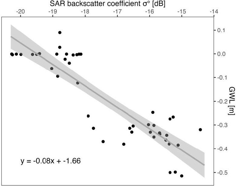
Correlation between synthetic aperture radar backscatter coefficient and groundwater level (gray line represents the regression line; gray area represents the confidence interval of 95%; linear model equation: y = −0.08x + −1.66)
Source: own work.
The peat subsidence (vertical displacement) rate, a remote sensing-derived parameter correlated with GWL, was also utilized in the model. The decline in GWL, leading to increased soil respiration, has been identified as a primary factor contributing to the acceleration of subsidence rates (Ma et al., 2022). The subsidence data were obtained from the study by Ghezelayagh et al. (2024), which employed the InSAR technique to measure the vertical displacement of the peat surface within the BbPN area. Changes in peat surface elevation using InSAR are estimated based on InSAR coherence, which is the correlation between two subsequent SAR images (Abdel-Hamid et al., 2021; Hrysiewicz et al., 2024) and can provide centimeter to millimeter precision (Hoyt et al., 2020). This parameter was categorized into three intervals: −0.05 to −0.02 m⋅year−1, −0.02 to −0.01 m⋅year−1 and −0.01 to 0.05 m⋅year−1 (Table 1).
The third parameter used to build the BBN was the distance to ditches, canals, or rivers. These data were compiled from digitized vector layers of watercourses within the BbPN and created through orthophoto mapping and field verification. The classification of this parameter was based on the meta-analysis by Bring et al. (2022), who identified specific thresholds for the impact of drainage on a peatland’s GWL. The study indicated that the effect of ditching on the GWL diminishes by 50% at a distance of 21 m and by 75% at 97 m relative to the immediate vicinity of the ditch. Moreover, the drainage effect is negligible beyond approximately 440 m. For the model, four distance classes were established based on the findings of this study, as outlined in Table 1.
All data were pre-processed in the ArcGIS 10.7.1 software. The remote sensing data, provided as raster layers, were spatially extracted to each point feature corresponding to the piezometer locations and their associated multi-year GWL records. The extracted values were subsequently classified according to the categories outlined in Table 1. This classification was a critical step, as BBNs utilize conditional probability tables, which are more effectively managed with discrete variables (Cobb et al., 2007). The BBN was built in GeNIe Academic Version 4.1 (BayesFusion, LLC) by learning the parameters. The network graphs presenting example results were exported from Netica 7.01 (Norsys Software Corp). The network structure was designed as depicted in Figure 3, where the remote sensing data serve as parent nodes, and the GWL acts as the child node. This configuration allows the model to estimate the probability of a specific GWL class occurring based on the provided remote sensing parameters. The model was trained using data from the whole Biebrza basin area.
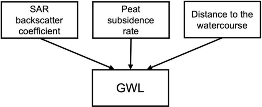
Conceptual model of the Bayesian belief network
Source: own work.
The Bayesian belief network’s probability results were analyzed using Microsoft Excel and RStudio Version 2023.12.0+369 (R Core Team, 2023). The packages used included ‘caret’ (Kuhn, 2008), ‘ggplot2’ (Wickham, 2016) and ‘Metrics’ (Hamner & Frasco, 2018). Unlike deterministic models, a BBN estimates the probability distribution of potential outcomes rather than predicting exact values. Due to limited data availability, two approaches for network validation were applied. The first approach involved creating 12 random polygons of 100 ha (Fig. 4A), each covering at least two piezometers, to calculate the mean GWL within each extent. The area percentage contribution of each model parameter class was then determined within each polygon. The second validation approach used 26 BbPN plots (cadaster-based, real parcels) with areas ranging from 0.9 ha to 450 ha, with an average of 42 ha (Fig. 4B). In the case of the BbPN plots, the GWL value for each plot was derived from either one piezometer or an average of several piezometers located within the polygon, depending on the number of piezometers intersecting the plot. Then, the percentage contribution of each model variable class (SAR backscatter coefficient, peat subsidence rate, and distance to watercourses) was used as an input in the Bayesian belief network to generate conditional probabilities of different classes of GWL. The class with the highest probability (referred to as a prediction or predicted class later in this study) was then compared with the class of the mean observed GWL at each polygon/plot. However, it should be stressed that the prediction from the model is not a deterministic value and is only one from the possible set of outcomes.
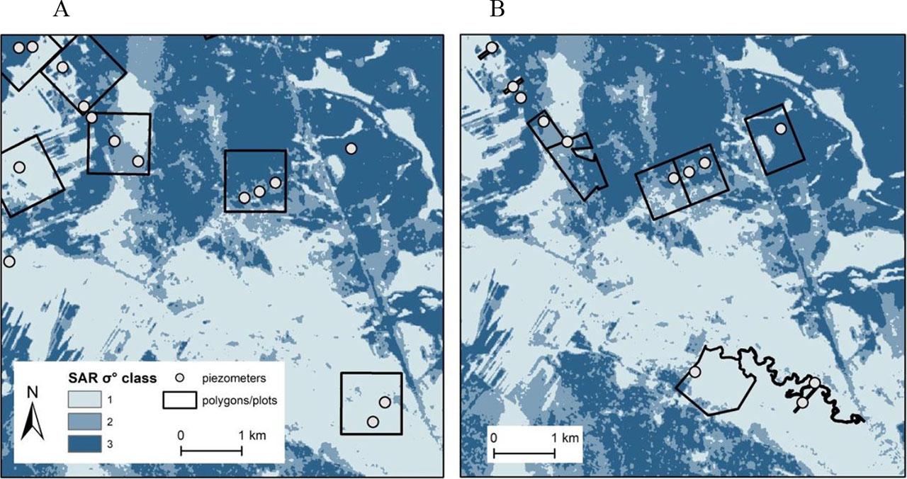
Maps showing 100-hectare polygons (A) and the Biebrza National Park plots (B) with a synthetic aperture radar backscatter coefficient raster layer as a background
Source: own work.
The model’s performance was assessed using a confusion matrix and predictive accuracy. The confusion matrix summarizes the model performance by comparing the predicted and actual classes and is a valuable tool for validating probabilistic models in classification tasks (Chen & Pollino, 2012; Marcot, 2012). The predictive accuracy was calculated as the ratio of correct predictions to the total number of predictions. Additionally, a sensitivity analysis, as sensitivity to findings specific to Bayesian networks (Rositano et al., 2017), was performed to determine which model variables had the most significant influence on the GWL prediction. The indicator used for the sensitivity analysis was entropy reduction, with entropy being a measure of uncertainty of variables (Villaverde et al., 2014).
The statistical independence of the model variables was evaluated. The Shapiro–Wilk test assessed whether the datasets conformed to the normal distribution assumption. The findings indicated that the SAR backscatter coefficient and distance to the watercourse data deviated from a normal distribution (p-value < 0.05), necessitating the application of the Spearman’s rank correlation coefficient to investigate the independence of the variables. The Spearman’s rank correlation coefficient (ρ) was −0.11 between SAR backscatter and subsidence, with a p-value of 0.47, indicating that there is no significant association between the variables in the dataset. Similarly, the test showed no correlation between SAR backscatter and distance to the watercourses (ρ = 0.11; p-value = 0.45) and between subsidence and distance (ρ = −0.03; p-value = 0.82), thus making these variables suitable to be used in the BBN approach (Table 2).
Spearman’s rank correlation results between model variables
| Pair of compared model variables | Spearman’s rank correlation parameters | |
|---|---|---|
| ρ | p-value | |
| Synthetic aperture radar backscatter coefficient–subsidence | −0.11 | 0.47 |
| Synthetic aperture radar backscatter coefficient–distance to the watercourses | 0.11 | 0.45 |
| Subsidence–distance to the watercourses | −0.03 | 0.82 |
Source: own work.
The model’s conditional probability table (CPT) generated 36 possible combinations of remote sensing classes. However, due to limited data, some combinations are not present in the model. Therefore, the model was tested using two approaches, as described in the “Data processing, building Bayesian network and statistical analyses” subsection. The percentage contributions of the model variables’ classes were calculated for each polygon and BbPN plot used for validation (Table 3). Based on these contributions, the distribution of probabilities of the occurrence of GWL classes was generated (Table 4). The BBNs for one 100-hectare polygon (Polygon 9) and one BbBN plot (Plot 26) selected randomly are shown in Figure 5 to present how the results are generated. Belief bars visually represent conditional probabilities on the BBN, which reflect the likelihood of different outcomes for the child node based on the contributions of the model parameters. In Polygon 9, the presented percentage contribution of the model parameters’ classes indicates that the GWL in class C5 (with a 58.2% probability) is most likely to occur within its boundaries. The probabilities of the GWL falling into classes C1, C2, C3, C4 and C6 are 6%, 10.3%, 5.5%, 15% and 5%, respectively. In Plot 26, the GWL in class C2 is most likely to occur (with a 50.3% probability). The probabilities for the GWL being in classes C1 and C3 are 23.9% and 11.7%, respectively. Additionally, the probability of the GWL being in classes C4, C5, and C6 is 4.7% for each.
Area percentage contributions of each model variables class in polygons and plots used for validation
| V.m. | No | Area [ha] | Avg. obs. GWL [m] | SAR backscatter coefficient class distribution [%] | Subsidence class distribution [%] | Distance to the watercourse class distribution [%] | |||||||
|---|---|---|---|---|---|---|---|---|---|---|---|---|---|
| 1 | 2 | 3 | 1 | 2 | 3 | 1 | 2 | 3 | 4 | ||||
| Polygon | 1 | 100 | −0.364 | 48.3 | 21.9 | 29.8 | 21.7 | 60 | 18.3 | 0 | 4 | 53.4 | 42.6 |
| 2 | 100 | −0.293 | 3.5 | 26.7 | 69.8 | 0.6 | 31.4 | 68 | 0 | 0 | 0 | 100 | |
| 3 | 100 | −0.391 | 6.6 | 11.9 | 81.5 | 64.3 | 34.6 | 1.1 | 3.6 | 10.4 | 71.6 | 14.4 | |
| 4 | 100 | −0.314 | 30.1 | 41.0 | 28.9 | 17.1 | 76 | 6.9 | 0 | 0 | 0 | 100 | |
| 5 | 100 | −0.309 | 23.2 | 22.8 | 54.0 | 11.1 | 57.2 | 31.7 | 0 | 0.7 | 35.3 | 64 | |
| 6 | 100 | −0.332 | 29.6 | 4.4 | 66.0 | 52.9 | 44.8 | 2.3 | 5.8 | 13.5 | 40.4 | 40.3 | |
| 7 | 100 | −0.001 | 96.0 | 4.0 | 0.0 | 24.3 | 65.6 | 10.1 | 10.6 | 23.4 | 66 | 0 | |
| 8 | 100 | −0.006 | 79.9 | 10.3 | 9.8 | 11 | 55.9 | 33.1 | 15.5 | 41.2 | 43.3 | 0 | |
| 9 | 100 | −0.004 | 81.5 | 13.6 | 4.9 | 63.3 | 35.6 | 1.1 | 0 | 0 | 3 | 97 | |
| 10 | 100 | −0.002 | 48.6 | 46,0 | 5.4 | 22.6 | 60.5 | 16.9 | 0.3 | 1.7 | 25.9 | 72.1 | |
| 11 | 100 | −0.109 | 79.8 | 6.6 | 13.6 | 22.6 | 65.2 | 12.2 | 0 | 0 | 14.1 | 85.9 | |
| 12 | 100 | −0.012 | 96.7 | 3.3 | 0.0 | 34.6 | 61.5 | 3.9 | 4 | 10.8 | 42.4 | 42.8 | |
| BbPN plot | 1 | 5.72 | −0.002 | 64.6 | 27.4 | 8 | 30 | 60 | 10 | 0 | 0 | 18.5 | 81.5 |
| 2 | 4.75 | −0.338 | 20.3 | 65.8 | 13.9 | 10 | 80 | 10 | 0 | 1.3 | 53.9 | 44.8 | |
| 3 | 1.41 | −0.5 | 10.7 | 44.3 | 45 | 33.3 | 66.7 | 0 | 13.6 | 45.5 | 40.9 | 0 | |
| 4 | 0.92 | −0.338 | 1.1 | 78.4 | 20.5 | 0 | 100 | 0 | 0 | 0 | 0 | 100 | |
| 5 | 1.74 | −0.351 | 6.9 | 24.7 | 68.4 | 33.3 | 66.7 | 0 | 0 | 0 | 100 | 0 | |
| 6 | 1.73 | −0.267 | 14.4 | 29.3 | 56.3 | 0 | 100 | 0 | 0 | 0 | 0 | 100 | |
| 7 | 7.21 | 0.001 | 100 | 0 | 0 | 33.3 | 41.7 | 25 | 22.5 | 25 | 52.5 | 0 | |
| 8 | 1.3 | −0.002 | 100 | 0 | 0 | 0 | 33.3 | 66.7 | 4.8 | 19 | 76.2 | 0 | |
| 9 | 53.24 | −0.304 | 19.3 | 56.1 | 24.6 | 1.1 | 47.8 | 51.1 | 0 | 0 | 0 | 100 | |
| 10 | 38.63 | −0.001 | 29.2 | 50.7 | 20.1 | 32.8 | 61.2 | 6 | 3.3 | 10.2 | 52.6 | 33.9 | |
| 11 | 18.46 | −0.003 | 76.7 | 23.3 | 0 | 9.1 | 63.6 | 27.3 | 0 | 0 | 0 | 100 | |
| 12 | 53.57 | −0.287 | 6.8 | 47.8 | 45.4 | 0 | 18.7 | 81.3 | 0 | 0 | 0 | 100 | |
| 13 | 50.47 | −0.314 | 2.6 | 46.9 | 50.5 | 18.9 | 71.1 | 10 | 0 | 0 | 0 | 100 | |
| 14 | 65.53 | −0.514 | 12.3 | 9.9 | 77.8 | 53.8 | 43.4 | 2.8 | 3.6 | 9.8 | 52.8 | 33.8 | |
| 15 | 19.53 | −0.247 | 0.7 | 73.6 | 25.7 | 5.7 | 80 | 14.3 | 0 | 0 | 0 | 100 | |
| 16 | 50.94 | −0.333 | 19.4 | 20.3 | 60.3 | 9 | 64 | 27 | 0 | 0 | 8.8 | 91.2 | |
| 17 | 39.29 | −0.372 | 4.7 | 10 | 85.3 | 57.1 | 42.9 | 0 | 2.1 | 8.9 | 76.1 | 12.9 | |
| 18 | 61.39 | −0.062 | 50.6 | 22.4 | 27 | 4.6 | 55 | 40.4 | 2.4 | 8.9 | 54.4 | 34.3 | |
| 19 | 87.01 | −0.005 | 87 | 10.1 | 2.9 | 31 | 65.2 | 3.8 | 2.3 | 7.5 | 50 | 40.2 | |
| 20 | 2.01 | −0.023 | 100 | 0 | 0 | 33.3 | 66.7 | 0 | 3.1 | 15.6 | 81.3 | 0 | |
| 21 | 450.55 | −0.001 | 90.3 | 5.2 | 4.5 | 44.3 | 51.1 | 4.6 | 2 | 4.8 | 21.4 | 71.8 | |
| 22 | 3.86 | −0.001 | 100 | 0 | 0 | 28.6 | 71.4 | 0 | 0 | 0 | 0 | 100 | |
| 23 | 41.17 | −0.001 | 86.5 | 10.7 | 2.8 | 13.7 | 64.4 | 21.9 | 21.9 | 47.7 | 30.4 | 0 | |
| 24 | 2.19 | −0.001 | 50.9 | 12.7 | 36.4 | 0 | 66.7 | 33.3 | 14.7 | 50 | 35.3 | 0 | |
| 25 | 1.78 | −0.001 | 44.3 | 19.9 | 35.8 | 0 | 66.7 | 33.3 | 14.3 | 35.7 | 50 | 0 | |
| 26 | 24.2 | −0.320 | 0 | 1.2 | 98.8 | 53.5 | 41.8 | 4.7 | 0 | 0 | 48.1 | 51.9 | |
V.m. – validation method; Avg. obs. GWL – average observed groundwater level; SAR – synthetic aperture radar; BbPN – Biebrza National Park.
Source: own work.
Conditional probabilities of groundwater level classes generated from the Bayesian belief network
| V.m. | No | Avg. obs. GWL [m] | GWL class probability [%] | GWL class | ||||||
|---|---|---|---|---|---|---|---|---|---|---|
| C1 | C2 | C3 | C4 | C5 | C6 | Obs. | Pred. | |||
| Polygon | 1 | −0.364 | 10 | 28.5 | 10.6 | 6.95 | 37.8 | 6.05 | C2 | C5 |
| 2 | −0.293 | 5.96 | 22.5 | 52 | 5.83 | 7.85 | 5.82 | C3 | C3 | |
| 3 | −0.391 | 20.8 | 50.8 | 7.07 | 5.87 | 9.66 | 5.79 | C2 | C2 | |
| 4 | −0.314 | 7.38 | 39.1 | 14 | 6.76 | 27 | 5.73 | C2 | C2 | |
| 5 | −0.309 | 10.6 | 34.4 | 20.8 | 6.52 | 21.4 | 6.19 | C2 | C2 | |
| 6 | −0.332 | 16.9 | 35.4 | 9.91 | 7.63 | 23.4 | 6.77 | C2 | C2 | |
| 7 | −0.001 | 6.94 | 8.55 | 7.25 | 6.94 | 59.7 | 10.6 | C5 | C5 | |
| 8 | −0.006 | 8.67 | 12.6 | 9.17 | 7.98 | 48.8 | 12.8 | C5 | C5 | |
| 9 | −0.004 | 6.02 | 10.3 | 5.52 | 15 | 58.2 | 4.99 | C5 | C5 | |
| 10 | −0.002 | 7.03 | 29.1 | 10.5 | 8.04 | 38.8 | 6.51 | C5 | C5 | |
| 11 | −0.109 | 6.17 | 13.5 | 8.09 | 7.99 | 59.4 | 4.89 | C4 | C5 | |
| 12 | −0.012 | 5.74 | 7.16 | 5.88 | 8.61 | 65.6 | 6.98 | C5 | C5 | |
| BbPN plot | 1 | −0.002 | 6.68 | 21 | 8.24 | 8.87 | 49.5 | 5.71 | C5 | C5 |
| 2 | −0.338 | 7.9 | 50.4 | 9.52 | 6.23 | 19.9 | 6.05 | C2 | C2 | |
| 3 | −0.500 | 14.2 | 34.2 | 16.6 | 9.9 | 14.7 | 10.4 | C1 | C2 | |
| 4 | −0.338 | 5.26 | 67.8 | 10.4 | 5.26 | 6.08 | 5.26 | C2 | C2 | |
| 5 | −0.351 | 20.6 | 56.2 | 4.64 | 4.64 | 9.24 | 4.64 | C2 | C2 | |
| 6 | −0.267 | 4.57 | 52.3 | 18.6 | 4.57 | 15.4 | 4.57 | C3 | C2 | |
| 7 | 0.001 | 7.75 | 7.75 | 7.75 | 7.75 | 55.2 | 14.2 | C6 | C5 | |
| 8 | −0.002 | 6.06 | 6.06 | 6.06 | 6.06 | 67.8 | 7.93 | C5 | C5 | |
| 9 | −0.304 | 6.49 | 30.2 | 32.1 | 6.44 | 18.4 | 6.4 | C2 | C3 | |
| 10 | −0.001 | 10.2 | 38.7 | 10.5 | 7.78 | 25.3 | 7.45 | C5 | C2 | |
| 11 | −0.003 | 5.72 | 15.6 | 8.9 | 7.11 | 57 | 5.72 | C5 | C5 | |
| 12 | −0.287 | 6.65 | 16.9 | 52.8 | 6.65 | 10.4 | 6.65 | C3 | C3 | |
| 13 | −0.314 | 9.32 | 49.5 | 20.8 | 6.24 | 7.95 | 6.14 | C2 | C2 | |
| 14 | −0.514 | 19.6 | 44.7 | 9.63 | 6.48 | 13.4 | 6.13 | C1 | C2 | |
| 15 | −0.247 | 6.51 | 56 | 18.9 | 6.03 | 6.52 | 6.02 | C3 | C2 | |
| 16 | −0.333 | 8.04 | 35.7 | 26.6 | 5.77 | 18.4 | 5.45 | C2 | C2 | |
| 17 | −0.372 | 21.7 | 52.8 | 6.65 | 5.35 | 8.17 | 5.3 | C2 | C2 | |
| 18 | −0.062 | 9.27 | 24.3 | 12.8 | 7.14 | 39 | 7.47 | C5 | C5 | |
| 19 | −0.005 | 6.14 | 11.8 | 6.24 | 7.86 | 61.6 | 6.37 | C5 | C5 | |
| 20 | −0.023 | 6.51 | 6.51 | 6.51 | 6.51 | 66.4 | 7.54 | C5 | C5 | |
| 21 | −0.001 | 5.81 | 8.9 | 5.78 | 10.9 | 63 | 5.61 | C5 | C5 | |
| 22 | −0.001 | 3.93 | 3.93 | 3.93 | 3.93 | 74.6 | 3.93 | C5 | C5 | |
| 23 | −0.001 | 8.24 | 10.6 | 9.72 | 8.08 | 47.8 | 15.6 | C5 | C5 | |
| 24 | −0.001 | 11.8 | 17.5 | 11.7 | 9.62 | 36.4 | 12.9 | C5 | C5 | |
| 25 | −0.001 | 12.1 | 22 | 11.5 | 9.08 | 33.5 | 11.9 | C5 | C5 | |
| 26 | −0.320 | 23.9 | 50.3 | 11.7 | 4.71 | 4.71 | 4.71 | C2 | C2 | |
V.m. – validation method; Avg. obs. GWL – average observed groundwater level; Obs. – observed; Pred. – predicted; BbPN – Biebrza National Park.
Source: own work.
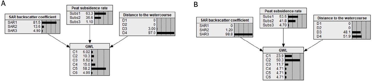
Example results from the Bayesian belief network: A – percentage contribution of model parameters in Polygon 9, B – percentage contribution of model parameters in Biebrza National Park Plot 26. Groundwater level node represents the results as a probability distribution of the occurrence of certain GWL classes
Source: own work.
The confusion matrices assessing the performance of the model for both sets of 100-hectare polygons and BbPN plots are shown in Figure 6. Diagonal elements on the matrix represent correctly predicted classes, while off-diagonal elements indicate misclassifications. Using 100-hectare polygons as a validation set, 10 out of 12 predictions were correct, resulting in a prediction accuracy of 83.3% (Fig. 6A). Validating the network with a set of BbPN plots resulted in an accuracy of 73.1%, where 19 out of 26 predictions were correct. Sensitivity analysis revealed that the entropy reduction was 0.315, 0.066, and 0.038 for SAR backscatter coefficient, distance to the watercourse, and peat subsidence rate, respectively. This means that the SAR backscatter coefficient is the parameter with the highest influence over the GWL result in the model.
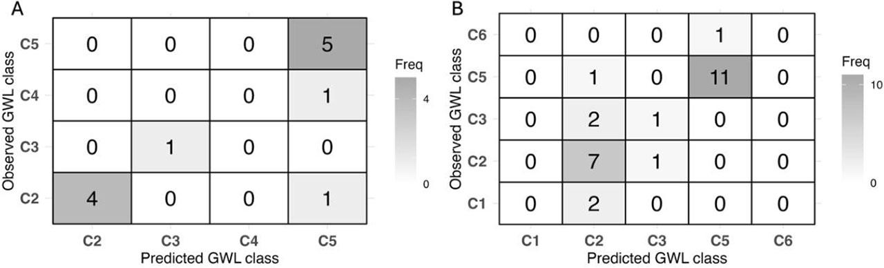
Confusion matrices displaying the number of matched and unmatched classes between predicted and actual groundwater level values for 100 ha polygons (A) and the Biebrza National Park plots (B) used as the validation set
Source: own work.
The results of this study highlight the potential of using BBN in conjunction with remote sensing data to address the challenge of estimating GWLs in peatlands, particularly in the context of environmental management and GHG mitigation. The model achieved predictive accuracies of 73.1–83.3%, proving its effectiveness as a cost-efficient alternative to traditional GWL measurement methods, which are often hindered by logistical constraints and high costs. The results demonstrate that remote sensing can serve as a reliable proxy for groundwater dynamics, which are vital for understanding and managing peatland ecosystems. These findings are particularly important as they provide a means to evaluate the hydrological status of peatlands that lack extensive monitoring infrastructures, ultimately supporting restoration efforts aimed at enhancing carbon sequestration in peat soils. By linking GWL estimates to GHG emissions, this research can contribute to the broader goal of developing adaptive management strategies that can support policy decisions and promote sustainable land use practices.
Numerous approaches have been explored to estimate GWLs in peatlands without direct measurements, often by testing a range of remote sensing and non--remote sensing indicators to identify the most accurate and sensitive proxies for GWL prediction (Kameoka et al., 2021; Georgiou et al., 2023). Some of them reached higher (Hikouei et al., 2023) or lower (Bechtold et al., 2014) accuracy, although they had much more input data to teach the model. However, a significant challenge emerges from upscaling these indicators and models for application beyond the specific environments where they were initially built. For instance, Adinugroho et al. (2021) developed a model using Indonesian peatlands to estimate soil moisture using Sentinel imagery as a proxy for groundwater level. This model is available as an open-source SEPAL tool (FAO, 2021), but it did not perform well in the peatlands in BbPN. Ideally, an extensive monitoring network across diverse types and conditions of peatlands would be required to provide spatially comprehensive GWL data, facilitating robust model development and validation. Unfortunately, establishing and managing such a network is generally not feasible due to the significant financial, time, and logistical resources required and the different monitoring protocols in peatlands across countries (Gutierrez Pacheco et al., 2021). The Bayesian belief network employed in this study faces similar challenges. Several uncertainties emerged during data preparation, model construction, and validation. A primary concern lies in the inherent limitations of remote sensing data, such as the constraints imposed by spatial resolution and satellite revisit intervals. Additionally, because synthetic aperture radar (SAR) cannot penetrate dense tree canopies, some datasets had to be excluded to prevent the introduction of inaccuracies. Further complications arise from temporal discrepancies between the multi-year GWL measurements and the remote sensing data, as these datasets were collected over differing timeframes. For instance, the SAR backscatter coefficient used in this study was averaged from all available Sentinel-1 imagery since its launch. In contrast, the multi-year GWL data from some piezometers represents a more extended period, potentially leading to inconsistencies. Other uncertainties arise from the limited size of the training dataset, which reduces the variety of variable class combinations within the model due to limitations in piezometer coverage, potentially leading to inaccurate predictions. The possibility of mismatching definitions of intervals or classes of variables aggravates this issue. The obtained accuracy in the built model may be somewhat misleading due to unbalanced proportions in the class distributions, as class C5 in the validation set was much more frequent than the others, and some classes were even missing (C1 and C3 in the 100-hectare polygon validation set). Moreover, it is crucial to address whether the level of accuracy in GWL prediction is sufficient for practical applications, such as estimating greenhouse gas emissions.
The most common way to teach Bayesian networks is using observational data and/or expert knowledge (Daly et al., 2011). However, the data is often insufficient to capture all model variables (Masegosa et al., 2016), which was the case in this study. One approach to addressing this issue would be to obtain missing data from other models. In terms of the future development of the BBN created in this study, there are plans to construct a multiple regression model. This model would facilitate the generation of new GWLs based on the known remote sensing parameters used in the study. The generated data could then be used to update the developed BBN. Additionally, the data from the BbPN area should be complemented and tested with data from other peatlands across all of Poland and outside of the country, especially since other studies found that results obtained at one peatland using SAR imagery cannot be compared with different sites (Lees et al., 2021). Incorporating data from various peatlands will improve the accuracy of future models and provide a more comprehensive understanding of the relationship between the GWL and parameters derived from remote sensing. Furthermore, the potential of other remote sensing data sources could also be investigated to improve the prediction accuracy.
Despite the indicated limitations, the presented assessment methodology may be one of the few that can be applied under operational conditions to determine the multi-year average GWL in peatlands, where necessary (e.g., for the purpose of assessing the hydrological status of remote/unmonitored peatlands before undertaking restoration measures) and where hydrological monitoring has never been conducted and the use of more complex methods will be pointless due to the long analysis time, its complexity and data requirements. Indeed, under the assumptions of implementing programs that encourage carbon retention in rewetted peat soils, there will be a need for an ex-ante evaluation of the effectiveness and scale of success of these measures. Under such conditions, a rapid assessment of the average state of groundwater will prove necessary. So far, published experience of the uncertainty in the success of peatland rewetting and the resulting increase in GWL of a few centimeters (Karimi et al., 2024) indicates that even an uncertainty-laden assessment of water levels using the Bayesian belief network presented here can become a useful, and perhaps even the only, tool that provides a meaningful quantification of peatland GWL from a multi-year period. However, this will certainly require calibration and verification of the method on other, possibly numerous, peatlands with available data from long-term GWL monitoring.
This research demonstrates the application of a BBN model integrated with remote sensing data to estimate the mean groundwater levels in peatlands, with a specific focus on the Biebrza National Park in Poland. The developed Bayesian network can predict GWLs within the defined classes with an accuracy of 73.1–83.3%. Additionally, dual-polarized radar backscatter has been validated as a proxy for GWL, showing a high correlation with field-measured GWL data. Among the remote sensing variables considered, the SAR backscatter coefficient was the most sensitive in predicting the GWL in peatlands. The study emphasizes the potential of the Bayesian network model as a cost-effective and efficient alternative to traditional GWL measurement techniques. It also highlights the critical role of high-resolution remote sensing data in improving GWL estimates and the effectiveness of Bayesian networks in managing uncertainties and providing conditional probabilities for different outcomes. This underscores the importance of the continued development and refinement of predictive models for environmental management. Developing this modeling approach to other peatland areas globally is recommended, particularly in regions where ground-based monitoring is logistically challenging or costly. Future research should also explore incorporating additional remote sensing parameters and the potential impact of climatic variables on the model’s predictive accuracy. In conclusion, the study demonstrates the feasibility and effectiveness of using Bayesian networks and remote sensing data to estimate GWLs in peatlands. This approach remains a valuable next step in achieving efficient peatland monitoring and management, despite its uncertainties. However, further improvements in the prediction of GWL by utilizing available hydrological and remote sensing data are required, especially including testing alternative modeling approaches.