Deterministic Blockmodeling of Two-Mode Binary Networks Using a Two-Mode KL-Median Heuristic

A relocation heuristic (RH)

A relocation heuristic (RH) for the DTMBP was developed by Doreian et al. (2004, 2005, Chapter 8). In its original design, the RH used two neighborhood search operations: (i) transfers of objects from one cluster to another; and (ii) exchanges of cluster memberships for pairs of objects. Brusco and Steinley (2011) found the second of these operations to be ineffective when RH was implemented in a multistart framework using a fixed time limit. More specifically, the computational requirement associated with the examination of all possible exchanges is high, which implies fewer restarts of the algorithm can be realized within any prescribed time limit. Based on this finding, we implement a version of the RH using only transfers (see also Brusco et al., 2013a). The precise steps of the relocation algorithm are described below. In addition to previously defined terms, the description uses flagR and flagC, to indicate, respectively, whether a successful relocation has been found for either row objects or column objects. Also, flag1 is an indicator to control termination of the algorithm if the current solution is locally-optimal with respect to all possible relocations of row and column objects.

• Step 0. Initialization. Input an initial K-cluster partition of the row objects, π, and an initial L-cluster partition for the column objects, ω. Compute g(π, ω) using equations (1) through (3).

• Step 1. Evaluate all transfers of row objects.

  • Step 1a. Set flag1 = 0, flagR = 0, i = 0, and go to Step 1b.

  • Step 1b. Set i = i + 1. If i > n, then go to Step 1i; otherwise, set h = h : i ∈ S_h and go to Step 1c.

  • Step 1c. If ∣S_h∣ > 1, then set k = 0 and go to Step 1d; otherwise, return to Step 1b.

  • Step 1d. Set k = k + 1 and go to Step 1e.

  • Step 1e. If k = h, then go to Step 1d; otherwise go to Step 1f.

  • Step 1f. If k > K, then go to Step 1b; otherwise go to Step 1g.

  • Step 1g. Set π′ = π\{S_h, S_k} ∪ {S_h \ {i}} ∪ {S_k ∪ {i}}, compute g(π′, ω), and then proceed to Step 1h.

  • Step 1h. If g(π′, ω) < g(π, ω), then set π = π′, flag1 = 1, flagR = 1, h = k, and return to Step 1d; otherwise return to Step 1d.

  • Step 1i. If flagR = 0, then proceed to Step 2; otherwise return to Step 1a.

• Step 2. Evaluate all transfers of column objects.

  • Step 2a. Set flagC = 0 and j = 0 and go to Step 2b.

  • Step 2b. Set j = j + 1. If j > m, then go to Step 2i; otherwise, set h = h : j ∈ T_h and go to Step 2c.

  • Step 2c. If ∣T_h∣ > 1, then set l = 0 and go to Step 2d; otherwise, return to Step 2b.

  • Step 2d. Set l = l + 1 and go to Step 2e.

  • Step 2e. If l = h, then go to Step 2d; otherwise go to Step 2f.

  • Step 2f. If l > L, then go to Step 2b; otherwise go to Step 2g.

  • Step 2g. Set ω′ = ω\{T_h, T_l} ∪ {T_h \ {j}} ∪ {T_l ∪ {j}}, compute g(π, ω′), and then proceed to Step 2h.

  • Step 2h. If g(π, ω′) < g(π, ω), then set ω = ω′, flag1 = 1, flagC = 1, h = l, and return to Step 2d; otherwise return to Step 2d.

  • Step 2i. If flagC = 0, then proceed to Step 3; otherwise return to Step 2a.

• Step 3. Termination check.

  If flag1 = 1, then return to Step 1a; otherwise, return π, ω, g(π, ω) and STOP.

The RH begins in Step 0 with the selection of an initial blockmodeling solution. This solution can be randomly-generated or produced via some other type of heuristic procedure (see Brusco et al., 2013a). A cycle through Step 1 provides a search of all possible relocations of the n row objects from their current cluster to each of the other K-1 clusters. Relocations that improve the objective function are accepted as they arise. The algorithm will continue cycling through its search of row-object relocations until no further improvement in the criterion function can be realized. At this point, control is passed to Step 2, where a similar process is implemented for column objects. The algorithm terminates in Step 3 when no relocations of row objects or column objects can further improve the objective function.

This formulation of RH is not without its limitations. First, a potential source of bias can accrue from column-object relocations that are not considered until all improvements via row-object relocations have been made. Second, as noted by Brusco et al. (2013a), the algorithm is left-biased in the sense that row objects are evaluated in their natural order (1, 2,…,n), as are column objects. Third, the evaluation of n(K-1) and m(L-1) relocations on each cycle of Steps 1 and 2, respectively, can be computationally demanding as n, m, K, and L increase. This can seriously limit the number of restarts of the RH that can be completed within a prescribed time limit.

A two-mode KL-median heuristic

We apply the TMKLMedH, an adaptation of a heuristic for two-mode KL-means partitioning that has proven effective in previous studies (Baier et al., 1997; Brusco & Doreian, 2015a, b; Brusco & Steinley, 2007a; Van Rosmalen et al., 2009; Vichi, 2001). The heuristic process is a direct extension of the classic K-means (or, as defined by Hansen and Mladenović (2001), H-means) clustering heuristic for one-mode data (Forgy, 1965; Steinhaus 1956). The heuristic is implemented via the following steps:

• Step 0. Randomly assign the row objects to K clusters to create the initial partition, π. Randomly assign the column objects to L clusters to create the initial partition, ω. Compute f* = f(π,ω).

• Step 1. Row-object reassignment.

  • Step 1a: Compute d_kl ∀ 1 ≤ k ≤ K and 1 ≤ l ≤ L.

  • Step 1b. Compute ${\alpha }_{ik}={\displaystyle \sum _{l=1}^L{\displaystyle \sum _{j\in T_l}\left|x_{ij}-d_{kl}\right|}}\forall 1\le i\le n$ and 1 ≤ k ≤ K.

  • Step 1c. Update π by setting $i\in S_k:{\alpha }_{ik}=\underset{1\le h\le K}{\min }\{{\alpha }_{ih}\}$, ∀ 1 ≤ i ≤ n.

  • Step 1d. If S_k = ∅ for any k (1 ≤ k ≤ K), then set $i\prime \in S_k:{\alpha }_{i\prime }=\underset{1\le i\le n}{\max }\{\underset{1\le h\le K}{\min }\{{\alpha }_{ih}\}\}$. Set α_{i ′k} = 0 and repeat this step as necessary to guarantee no empty clusters.

• Step 2. Column-object reassignment.

  • Step 2a: Compute d_kl ∀ 1 ≤ k ≤ K and 1 ≤ l ≤ L.

  • Step 2b. Compute ${\text{β}}_{jl}={\displaystyle \sum _{K=1}^K{\displaystyle \sum _{i\in S_k}\left|x_{ij}-d_{kl}\right|}}\forall 1\le j\le m$ and 1 ≤ l ≤ L.

  • Step 2c. Update ω by setting $j\in T_l:{\beta }_{jl}=\underset{1\le h\le L}{\min }\{{\beta }_{jh}\}$, ∀ 1 ≤ j ≤ m.

  • Step 2d. If T_l = ∅ for any l (1 ≤ l ≤ L), then set $j\prime \in T_l:{\beta }_{ji}=\underset{1\le j\le m}{\max }\{\underset{1\le h\le L}{\min }\{{\beta }_{jh}\}\}$. Set β_{j ′l} = 0 and repeat this step as needed to guarantee no empty clusters.

• Step 3. Compute f(π,ω). If f(π,ω) < f*, then set f* = f(π,ω) and return to Step 1; otherwise, stop.

The heuristic begins with the random assignment of row objects and column objects to clusters in Step 0. Step 1 is a refinement process that, holding the column assignments fixed, assigns row objects to their best cluster based on minimum deviation from the current submatrix medians. Step 2 is similar, but holds the row assignments fixed and reassigns the column objects. The algorithm terminates in Step 3 when a complete cycle through Steps 1 and 2 does not produce an improvement in the criterion function value. Because of the potential for empty clusters after Steps 1c and 2c, Steps 1d and 2d are positioned to rectify this problem by reassigning the row object or column object that is farthest from its current cluster centroid to fill the empty cluster.

The TMKLMedH is sensitive to the initial partitions in Step 0 and does not necessarily converge to a globally-optimal solution for the problem posed in Equation (3). As with RH, a common practice is to restart the algorithm many times using different random initial partitions in Step 0, and selecting the results from a restart that produces the best value of the criterion function (see Brusco & Doreian, 2015a, b; Brusco & Steinley, 2007a; Van Rosmalen et al., 2009). This multistart restart practice was adopted in our implementation.

Experimental design

We conducted a simulation-based comparison of RH and TMKLMedH across test problems that were generated through the manipulation of eight design features: (i) number of row objects (n); (ii) number of column objects (m); (iii) number of row-object clusters (K); (iv) the number of column-object clusters (L); (v) the relative sizes of the row-object clusters; (vi) the relative sizes of the column-object clusters; (vii) the density of the image matrix; and (viii) the strength of the null and complete blocks. Two levels of each design feature were considered, resulting in a total of 2⁸ = 256 experimental cells. Three replicates were generated for each cell, resulting in a total of 768 test problems.

The two levels for the first design feature were n = 180 and n = 540. Likewise, for the second design feature, the levels were m = 180 and m = 540. The justification for these settings is based on several factors. First, we wanted the test problems to be large enough to discover real differences in performance between RH and TMKLMedH; hence, the lower settings of n = 180 and m = 180 are more than 50% larger than the highest setting used in similar research designs implemented by Brusco and Steinley (2007a) and Brusco et al. (2013a). Second, we wanted to keep the test problems of a sufficiently modest size to allow for the completion of the experiment within a reasonable time; hence we capped problem size at n = m = 540. Third, by separating n and m into distinct design features, we are able to look at problem instances where n and m are equal, as well as instances where n it three times larger than m (and vice versa).

The two levels for the third design feature were K = 3 and K = 6. Likewise, for the fourth design feature, the levels were L = 3 and L = 6. These are the same settings used in a two-mode blockmodeling simulation study conducted by Brusco and Steinley (2007a). Although these settings seem modest at first glance, it is important to remember that the simulation study considers all possible crossings of K and L. Therefore, the total number of clusters is either six (when K = L = 3), nine (where K= 6 and L = 3, or K = 3 and L = 6), or 12 (when K = L = 6). The total number of blocks that is established from these settings exhibits even greater variation, assuming values of nine (when K = L = 3), 18 (where K= 6 and L = 3, or K = 3 and L = 6), or 36 (when K = L = 6).

The two levels for the fifth design feature were: (i) an equal distribution of the row objects across the row clusters; and (ii) 60% of the row objects in one row cluster and an equal distribution of row objects across the remaining row clusters. The same two levels were used for the sixth design feature, which corresponded to the distribution of column objects across column clusters. These settings for distributions of objects across clusters are common in both the general clustering literature (Milligan, 1980) and the two-mode blockmodeling literature (Brusco & Doreian, 2015a; Brusco & Steinley, 2007a).

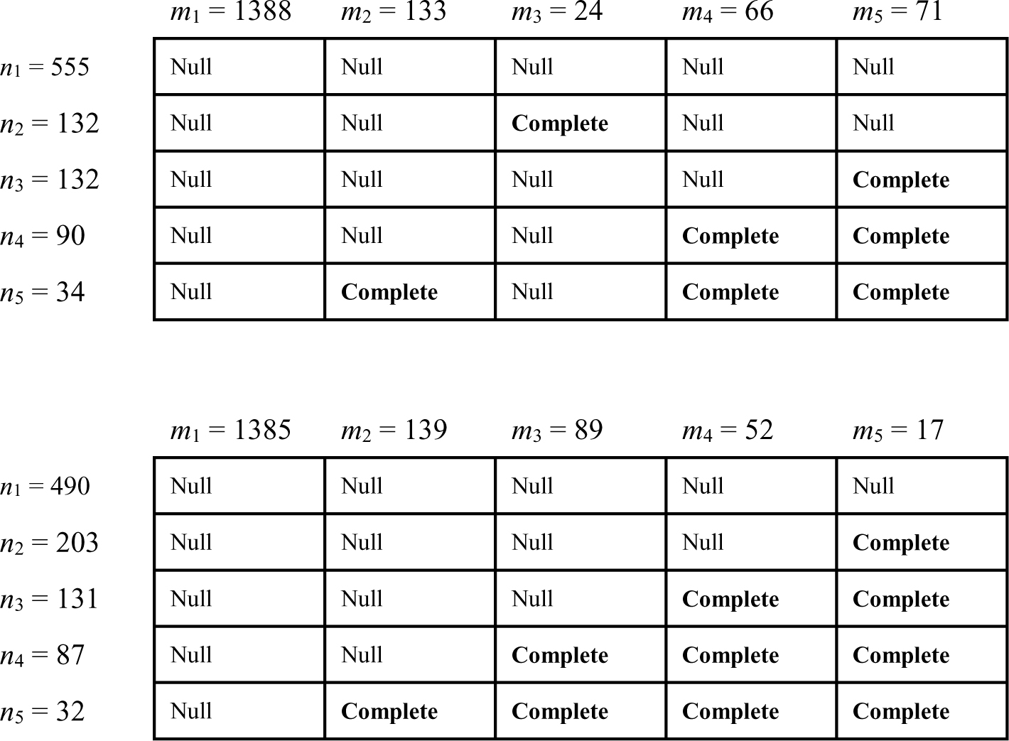
The seventh design feature pertained to the density of the image matrix. The image matrix, A = [a_kl], is a K × L binary matrix containing ones for the locations of complete blocks and zeros in the locations of null blocks in the ideal block structure. So, for example, if a_kl = 1, the submatrix formed by the row objects in row cluster k and the column objects in column cluster l should be complete to the greatest extent possible (more ones than zeros). At the first setting of this design feature, the image matrix density was 33% (i.e., one-third of the elements of the image matrix were ones and the other 2/3 were zeros). For the second setting, the image matrix density was 66%.

The eighth design feature pertained to the strength of the null and complete blocks. Under perfect structural equivalence, the null and complete blocks would have 100% zeros and ones, respectively. However, the generation of such problems would be much too easy for the algorithms. Even reducing the percentage to 90% or 80% was judged insufficient to differentiate between the algorithms. Therefore, the two settings for the eighth design feature were 70% and 60%. For example, at the 70% setting, complete blocks in the image matrix were generated to have roughly 70% ones and 30% zeros, whereas null blocks were generated to have roughly 70% zeros and 30% ones. At the 60% setting of the design feature, the strength of the blocks was further weakened, which tends to make the problems more formidable for the algorithms.

Implementation and performance measures

The RH and TMKLMedH algorithms were programmed in Fortran 90 and implemented on a desktop computer with an Intel ® Core^TM i7-4790 CPU @ 3.6GHz with 8 GB of RAM. Both algorithms were allotted a fixed time limit of three CPU minutes per test problem. For each test problem, the following performance measures were collected: (i) the value of the criterion function; (ii) the total number of restarts realized within the time limit; (iii) the adequacy of the recovery of the underlying cluster structure of the row objects, as measured by the adjusted Rand index (ARI: Hubert & Arabie, 1985); and (iv) the adequacy of the recovery of the underlying cluster structure of the column objects as measured by the ARI.

There are two performance measures in the simulation study that are particularly important. One is value of the criterion function as the minimized value is sought. The second is the extent to which the real partition structure is identified as captured by the ARI values. Accordingly, our primary emphasis is on these measures. We knew in advance that TMKLMedH would have far more restarts than RH within the allotted time limit. However, we did not know how the ratio of the numbers of restarts for these two algorithms would behave as a function of n, m, K, and L. Therefore, the number of restarts was stored to shed light on this issue. Although our emphasis is on the ability of TMKLMedH and RH to optimize the criterion that they seek to optimize, it is critical to also measure cluster recovery. We report ARI information for the recovery of underlying structure of row and column clusters. The ARI assumes a value of zero for chance agreement and a value of one for perfect agreement. We use Steinley’s (2004) recommendation regarding the interpretation of the adequacy of ARI values regarding pairs of partitions of the same network

Simulation results

The key finding of the simulation study was that TMKLMedH always produced a criterion function that was as good as or better than the criterion function for RH. Considering this finding, we focus on two measures for the comparison of the criterion functions obtained by the two algorithms: (i) MPRCF: the mean percentage reduction in the criterion function realized from using TMKLMedH instead of RH; and (ii) MPBetter: the mean percentage of test problems for which TMKLMedH found a better criterion function than RH. Table 1 reports MPRCF and MPBetter for the complete set of 768 test problems, as well as for each level of each design feature.

Table 1.

Simulation results: (i) MPICF: mean percentage improvement in the criterion function realized from using TMKLMedH instead of RH; (ii) MPbetter: Mean percentage of test problems for which TMKLMedH provided a better criterion function value than RH; (iii) MRR: mean ratio of the number of restarts for TMKLMedH to the number for RH within the three-minute time limit; and (iv) ARI recovery measures for row and column clusters for RH and TMLKMedH.

1 Note – the overall averages and the results for the design features with the two biggest effects in each column are highlighted for emphasis.

Across the complete set of 768 test problems, TMKLMedH produced a blockmodel with a better criterion function value than the one obtained by RH for 347 (47.786%) of the 768 test problems (i.e., MPBetter = 47.786%). Likewise, across all test problems, the mean improvement in the criterion function resulting from the use of TMKLMedH instead of RH was MPRCF = .344%, with a maximum improvement of 4.672%. Table 1 reveals that the number of row (K) and column (L) clusters were the design features associated with the greatest importance for revealing performance distinctions between the two methods. For example, at the setting of K = 3, the measured results were MPBetter = 29.167% and MPRCF = .039%. However, at K = 6, the corresponding measures were MPBetter = 66.406% and MPRCF = .649%. Similar findings are observed when comparing the MPBetter and MPRCF results for L = 3 and L = 6.

The superior performance of TMKLMedH stems from getting far more restarts than RH within the same time limit. Across the 768 test problems, the minimum, mean, and maximum ratios of the number of TMKLMedH restarts to RH restarts were 3.0, 24.8, and 72.2, respectively. Table 1 shows the mean ratio of restarts (MRR) was most strongly affected by the design features corresponding to the number of row (n) and column (m) objects. At the setting of n = 180, the MRR was 20.5; yet, at the setting of n = 540, the MRR was 29.1. Also, the MRR values for m = 180 and m = 540 were 18.5 and 31.1, respectively.

We turn our attention to the recovery of the cluster structures of the row and column objects. Across the 768 test problems, the average ARI values for row objects were .745 and .831 for RH and TMKLMedH, respectively. The average ARI values for column objects (.741 for RH and .829 for TMKLMedH) were markedly like those of the row objects. These differences are nontrivial, as the TMKLMedH averages exceed the threshold for good recovery of 0.8 recommended by Steinley (2004). In contrast, the RH averages seldom met this threshold. The ARI results in Table 1 reveal the superior recovery of TMKLMedH was systematic across most design feature levels. The two exceptions are the recovery of the row-cluster structure when K = 3 and the recovery of the column cluster structure when L = 3. For these two conditions, the recovery of both methods is outstanding, with average ARI values in the .96 to .97 range. By contrast, the results at K = 6 and L = 6 reveal the sharpest superiority of cluster recovery for TMKLMedH relative to RH. Table 1 also shows TMKLMedH as providing much stronger average recovery of row-cluster structure (column-cluster structure) than RH under the 60% density condition for row (column) clusters.

United Nations General Assembly (UNGA) Voting Data

Our first example for demonstrating the TMKLMedH uses United Nations General Assembly voting data, originally compiled by Doreian et al. (2013). Two network matrices were analyzed. The first was a 141 × 276 binary network matrix pertaining to votes of 141 countries on 276 ideological resolutions. The second was a 153 × 129 matrix for the votes of 153 countries on 129 military resolutions. Brusco et al. (2013a) performed a comparison of the performance of three two-mode blockmodeling algorithms on these two networks: (i) the relocation heuristic (RH) described in Section 3; (ii) a tabu search (TS) heuristic developed by Brusco and Steinley (2011); and (iii) a variable neighborhood search (VNS) heuristic developed by Brusco et al. (2013a) for two-mode blockmodeling. Each algorithm was applied to these network matrices for all numbers of clusters in the intervals 2 ≤ K ≤ 7 and 2 ≤ L ≤ 7. For each combination of K and L, the algorithms were constrained to a time limit of 10 CPU minutes on a 2.2 GHz Pentium 4 PC with 1 GB of RAM. There was little difference in the performance of the three methods for problems where K < 4 and/or L < 4. This suggests few differences for smaller t-mode binary networks.

For comparison to the results obtained by Brusco et al. (2013a), we ran the TMKLMedH heuristic for all combinations of 4 ≤ K ≤ 7 and 4 ≤ L ≤ 7 on both networks using the same 10-minute time limit on the same 2.2 GHz Pentium 4 PC with 1 GB of RAM. These ranges for K and L resulted in 16 test problems for each of the military and ideological networks, and a total of 32 problems overall. A comparison of the results for the four methods is displayed in Table 2.

Table 2.

Comparison of criterion function values for the UNGA networks.

Design feature levels	MPICF	MPbetter	MRR	RH (Row-ARI)	TMKLMedH (Row-ARI)	RH (Col-ARI)	TMKLMedH (Col-ARI)
Overall average	.344	47.786	24.824	.745	.831	.741	.829
n = 180 row objects	.264	48.698	20.543	.748	.810	.715	.778
n = 540 row objects	.425	46.875	29.105	.741	.852	.767	.880
m = 180 column objects	.300	50.521	18.512	.710	.779	.736	.807
m = 540 column objects	.388	45.052	31.136	.780	.853	.746	.850
K = 3 row clusters	.039	29.167	23.709	.967	.966	.695	.791
K = 6 row clusters	.649	66.406	25.938	.523	.696	.787	.866
L = 3 column clusters	.038	29.948	21.900	.698	.790	.968	.968
L = 6 column clusters	.651	65.625	27.747	.792	.872	.514	.690
Even row cluster density	.280	41.146	27.886	.785	.817	.765	.849
60% row cluster density	.409	54.427	21.762	.705	.845	.717	.808
Even column cluster density	.240	41.667	28.412	.771	.853	.788	.820
60% column cluster density	.449	53.906	21.236	.719	.809	.694	.837
33% Image matrix density	.367	48.438	26.753	.745	.829	.740	.830
66% Image matrix density	.321	47.135	22.895	.744	.833	.742	.827
70% block strength	.364	26.042	24.647	.808	.911	.804	.911
60% block strength	.325	69.531	25.001	.682	.751	.678	.747

1 Note: The criterion function values for the RH, TS, and VNS methods were taken from the article by Brusco et al. (2013a, Tables 2 and 3, pp. 204-205). The cell values shown in bold font reflect instances where the heuristic method failed to match the best criterion function value found across all four methods

The results in Table 2 are quite surprising. Across the 32 test problems, TMKLMedH matched the best-found criterion function value for 31 of the 32 test problems. By contrast, the TS, VNS, and RH methods only matched the best-found criterion function value for 24, 24, and 17 of the test problems, respectively. It is also noteworthy that, for three test problems (military resolution network with K = 7 and L = 4, ideological network with K = 4 and L = 7, and ideological network with K = 7 and L = 5), TMKLMedH obtained a new best-found criterion function value never matched by any of the other three methods.

We also collected, for each test problem, the elapsed time for TMKLMedH to find its best-found solution. For 22 of the 32 problems, TMKLMedH found its best solution within the first minute of its allotted 10-minute time limit. Moreover, there were only three problems where the best-found solution was not realized until after five minutes of elapsed time.

To summarize, the results using the UNGA data strongly support the simulation study. The TMKLMedH yielded a better criterion function value than RH for 15 problems, and the same criterion function value for the remaining 17 problems. The RH never produced a better result than TMKLMedH within the allotted time. Although the performance of TMKLMedH relative to TS and VNS is very favorable, considerable care is warranted. The TS and VNS procedures use relocation heuristics in their implementation and, therefore, are significantly slower than TMKLMedH. If the TS and VNS algorithms were redesigned to use the same process of finding medians and reassigning cases, perhaps their performances could improve substantially.

MovieLens Data

The second comparison of RH and TMKLMedH for a real-world network was undertaken using movie-rating data from the MovieLens database (Harper & Konstan, 2015). This data was retrieved from the KONECT (the Koblenz Network Collection: http://konect.uni-koblenz.de/networks/) website. Although the edges of the available network are weighted to reflect the ratings, our binary adaptation consists of n = 943 individuals who either did (x_ij = 1) or did not (x_ij = 0) provide ratings for each of m = 1682 movies. This network is less dense (density of 6.3%) than the UNGA networks.

We ran the RH and TMKLMedH algorithms for all combinations of 2 ≤ K ≤ 7 row clusters and 2 ≤ L ≤ 7 column clusters. Again, the algorithms were implemented on the desktop computer with an Intel ® Core^TM i7-4790 CPU @ 3.6GHz with 8 GB of RAM, but with a 10-minute time limit for all combinations of K and L. The results are summarized in Table 3.

Table 3.

Comparison of criterion function values and number of restarts for the MovieLens network.

		UNGA Military resolutions network				UNGA Ideological resolutions network
K	L	TMKLMedK	RH	TS	VNS	TMKLMedH	RH	TS	VNS
4	4	1743	1743	1743	1743	4220	4220	4220	4220
4	5	1730	1730	1730	1730	4144	4144	4144	4144
4	6	1730	1730	1730	1730	4136	4136	4144	4136
4	7	1730	1730	1730	1730	4131	4136	4136	4136
5	4	1713	1713	1713	1713	4200	4200	4200	4200
5	5	1663	1663	1663	1663	4020	4020	4020	4020
5	6	1649	1657	1649	1649	3947	3950	3947	3947
5	7	1646	1650	1646	1649	3890	3896	3947	3890
6	4	1707	1707	1709	1709	4194	4198	4194	4196
6	5	1633	1633	1633	1633	4001	4001	4001	4001
6	6	1614	1619	1612	1612	3841	3841	3841	3841
6	7	1599	1613	1608	1599	3763	3772	3763	3763
7	4	1702	1707	1707	1707	4194	4194	4194	4196
7	5	1627	1634	1627	1630	3997	4001	3999	3998
7	6	1577	1588	1577	1577	3822	3822	3825	3822
7	7	1565	1566	1565	1565	3691	3695	3691	3691

1 Note: PICF is the percentage improvement in the criterion function from using TMKLMedH instead of RH.

Table reveals that TMKLMedH produced a better criterion function value than RH for 30 of the 36 combinations of K and L. The two algorithms obtained the same criterion function value for the remaining six combinations. Across the 36 combinations of K and L, the average percentage improvement in the criterion function value resulting from the use of TMKLMedH instead of RH was .267%, and the maximum improvement was 2.309%. Again, the relative superiority of TMKLMedH stemmed from the fact that it accumulated far more restarts within the 10-minute time limit. Across the 36 test problems, the minimum, average, and maximum ratios of the number of TMKLMedH restarts to the number of RH restarts were 1.2, 20.7, and 35.6, respectively.

We recognized that the small percentage differences in the criterion values obtained by TMKLMedH and RH might not necessarily translate into meaningful differences with respect to blockmodel interpretation. The first step in this process was to select appropriate values for K and L to facilitate a comparison. Several criteria for selecting K and L have been proposed in the literature, such as examination of the number of local optima (Brusco et al., 2013b) and the Chull procedure (Brusco, Doreian, & Steinley, 2016; Ceulemans & Van Mechelen, 2005; Wilderjans, Ceulemans, & Meers, 2013). In this application, we use a visual aid for choosing K and L that is based on the use of heatmaps for the criterion values obtained by RH and TMKLMedH at different combinations of K and L.

Heatmaps for the criterion function values obtained by RH and TMKLMedH are displayed in Figure 1. These heatmaps were produced using the conditional formatting capabilities in Microsoft Excel using a red-yellow-green color scheme. Deep red values reflect the poorest of the criterion function values obtained, whereas deep greens signify the finest of the criterion values obtained. The progression in the heatmaps from red to reddish-yellow to yellow (and from yellow to greenish-yellow to green) visually illustrates improvement in the criterion function.

Figure 1.

An examination of the heatmaps in Figure 1 reveals some similarities and differences. Both heatmaps show deep red cells in the first row (K = 2) and first column (L = 2). This reflects the fact that very little (if any) improvement can be achieved by increasing K when L = 2, or by increasing L when K = 2. In a similar manner, both heatmaps show a deep yellow in the row for K = 3 (when L ≥ 3), as well as the column for L = 3 (when K ≥ 3). For conditions where K ≥ 4 and L ≥ 4, both heatmaps show shades of green, but to somewhat different extents. For example, a fairly sharp green begins to appear in the TMKLMedH heatmap at K = 5 and L = 5, and we used this as motivation for selecting the K = 5 and L = 5 solution for interpretation. By contrast, the green at K = 5 and L = 5 is not as sharp for the RH heatmap. Thus, if an analyst were looking at only the RH heatmap, a different K and L combination might be selected. This possibility of a different choice for K and L depending on whether RH or TMKLMedH is used is not unique to heatmaps, but could also occur for criteria such as the number of local optima or the rules used in the Chull procedure.

The criterion function values for RH and TMKLMedH at K = 5 and L = 5 were 87146 and 86498, a difference of less than one percent. However, for this same combination of K and L, the agreement between the RH and TMKLMedH partitions of the n = 943 individuals rating the movies was only ARI = .382. Similarly, the agreement between the partitions of the m = 1682 movies that were rated was ARI = .571. Both ARI measures fall to far below the 0.65 threshold for even fair agreement as recommended by Steinley (2004). Figure 2 helps to further clarify the distinctions between the RH and TMKLMedH blockmodels by providing their image matrices and cluster sizes. The image matrix in Figure 2 uses the term complete to signify blocks with greater than 50% density and null to indicate those with less than 50% density.

Figure 2.

The most striking similarity of the blockmodels obtained by RH and TMKLMedH is that each has one large cluster of individuals and one large cluster of movies that are loosely tied to the network (i.e., not associated with any complete blocks). However, once these two large clusters are accounted for, it is evident that TMKLMedH does a better job of identifying relationships between the remaining individuals and movies. The clean, interpretable structure of TMKLMedH is evidenced by the presence of all complete blocks below the main diagonal of its image matrix. This means that the five clusters of individuals associated with the TMKLMedH blockmodel were strongly tied to 0, 1, 2, 3, and 4 clusters of movies, respectively. Likewise, the five clusters of movies associated with the TMKLMedH blockmodel were strongly tied to 0, 1, 2, 3, and 4 clusters of individuals, respectively. The RH blockmodel does not have this structure. For example, TMKLMedH identified a cluster of n ₅ = 32 individuals who form complete blocks with the four latter clusters of movies. By contrast, RH did not identify such a cluster of individuals. In a similar manner, TMKLMedH obtained a cluster of m ₅ = 17 movies that form complete blocks with the four latter clusters of individuals. Again, RH did not identify such a cluster of movies.

Conclusions

Summary

We have introduced a model known as two-mode KL-median partitioning. It is similar to the well-established two-mode KL-means partitioning problem (Baier et al., 1997; Brusco & Steinley, 2007; Brusco & Doreian, 2015a, b; Hansohm, 2002; Trejos & Castillo, 2000; Van Rosmalen et al., 2009), but differs, as the criterion function is based on absolute deviations from submatrix medians instead of squared deviations from submatrix means. We discovered an interesting aspect of the two-mode KL-median criterion function: for binary network matrices, it is identical to a well-known criterion from the social network literature for the deterministic two-mode blockmodeling problem (DTMBP) based on structural equivalence (Brusco & Steinley, 2007, 2011; Doreian et al., 2004, 2005). The result is that a two-mode KL-median heuristic (TMKLMedH) can serve as a direct competitor to a relocation heuristic from the literature (RH). We also noted that the relationship between TMKLMedH and RH is analogous to the relationship between H-means and K-means clustering (Brusco & Steinley, 2007b; Hansen & Mladenović, 2001; Späth, 1980).

Several comparisons of TMKLMedH and RH were undertaken. The first comparison was based on a simulation experiment that showed TMKLMedH dramatically outperformed RH regarding criterion function values and partition recovery. The superior performance of TMKLMedH can be attributed to it realizing anywhere from 3 to 72 times more restarts than RH within the same three-minute time limit. The second evaluation based on previously published results for RH (and two other procedures) for two UNGA voting networks (Brusco et al., 2013a; Doreian et al., 2013). They revealed TMKLMedH as always outperforming RH. Moreover, TMKLMedH also outperformed both the tabu search and variable neighborhood search heuristics evaluated by Brusco et al. (2013a). Finally, TMKLMedH and RH were applied to a larger two-mode network from the KONECT database. The results reinforced the findings from the simulation and UNGA analyses, but also showed that the improvements realized from TMKLMedH relative to RH could lead to salient differences with respect to model selection and blockmodel interpretation.

Limitations and extensions

Some limitations and extensions associated with the research presented in this paper can broadly be divided into three categories: (i) restriction of our attention to binary two-mode networks; (ii) limitations of the algorithmic and experimental implementations; and (iii) the issue of metaheuristics.

As noted in Sections 1 and 2, a key focus of this paper showed TMKLMedH as a direct competitor for RH for binary network matrices. However, TMKLMedH is not restricted to binary network data. For example, TMKLMedH could be directly applied to the movie rating data using the actual 1 to 5 ratings as weighted edges. In fact, in circumstances where edge weights are restricted to a narrow range, TMKLMedH could well be an effective alternative to the two-mode KL-means partitioning methods described by Brusco and Doreian (2015a, b)

The RH and TMKLMedH algorithms were both written in Fortran 90 and programmed using similar conventions. Nevertheless, it is possible that the programming of the same algorithms by other researchers on different software platforms could results in different findings with respect to the number of restarts within the prescribed limits. Moreover, it is reasonable to expect that, as the time limits are increased, the relative performance differences between RH and TMKLMedH are apt to shrink. Nevertheless, we are confident about the general findings of our simulation experiment and real-world examples being sound. The TMKLMedH is much faster than RH and allows for many more restarts within a specified time constraint. This is likely to be important for larger, more computationally demanding networks.

While RH and TMKLMedH were identified as competitors for the DTMBP problem, however, the use of a metaheuristic approach uses the two methods in tandem may have additional value. Such a pairing of the two methods would mimic the HK-means procedure combining H-means and K-means for within-cluster sum-of-squares partitioning (see Brusco & Steinley, 2007b; Hansen & Mladenović, 2001). We are not touting TMKLMedH as superior to previously published methods, such as tabu search (Brusco & Steinley, 2011) and variable neighborhood search (Brusco et al., 2013a). However, we do maintain that the computational efficiency of these latter methods might be significantly improved if the relocation heuristic was replaced with the two-mode K-median partitioning approach.

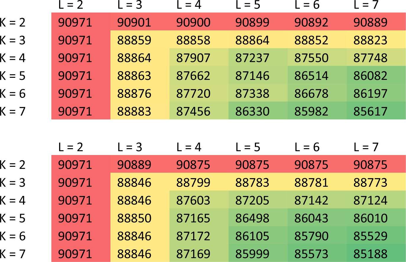
		Criterion function values			Number of restarts
K	L	TMKLMedH	RH	PICF	TMKLMedH	RH	RatioTMKLMedH / RH
2	2	90971	90971	0.000	2000	342	5.848
2	3	90889	90901	0.013	1980	201	9.851
2	4	90875	90900	0.028	1863	171	10.895
2	5	90875	90899	0.026	1799	129	13.946
2	6	90875	90892	0.019	1749	113	15.478
2	7	90875	90889	0.015	1687	103	16.379
3	2	90971	90971	0.000	1494	129	11.581
3	3	88846	88859	0.015	1345	86	15.640
3	4	88799	88858	0.066	1176	80	14.700
3	5	88783	88864	0.091	1130	59	19.153
3	6	88781	88852	0.080	1109	56	19.804
3	7	88773	88823	0.056	1111	52	21.365
4	2	90971	90971	0.000	1218	86	14.163
4	3	88846	88864	0.020	1079	57	18.930
4	4	87603	87907	0.347	936	42	22.286
4	5	87205	87237	0.037	893	42	21.262
4	6	87142	87550	0.468	806	36	22.389
4	7	87124	87748	0.716	782	36	21.722
5	2	90971	90971	0.000	1041	68	15.309
5	3	88850	88863	0.015	897	42	21.357
5	4	87165	87662	0.570	779	34	22.912
5	5	86498	87146	0.749	747	33	22.636
5	6	86043	86514	0.547	680	28	24.286
5	7	86010	86082	0.084	647	24	26.958
6	2	90971	90971	0.000	897	56	16.018
6	3	88846	88876	0.034	784	32	24.500
6	4	87172	87720	0.629	673	29	23.207
6	5	86105	87338	1.432	651	24	27.125
6	6	85790	86678	1.035	597	21	28.429
6	7	85529	86197	0.781	567	18	31.500
7	2	90971	90971	0.000	792	46	17.217
7	3	88846	88883	0.042	690	30	23.000
7	4	87169	87456	0.329	603	22	27.409
7	5	85999	86330	0.385	572	20	28.600
7	6	85573	85982	0.478	511	15	34.067
7	7	85188	85617	0.504	498	14	35.571