
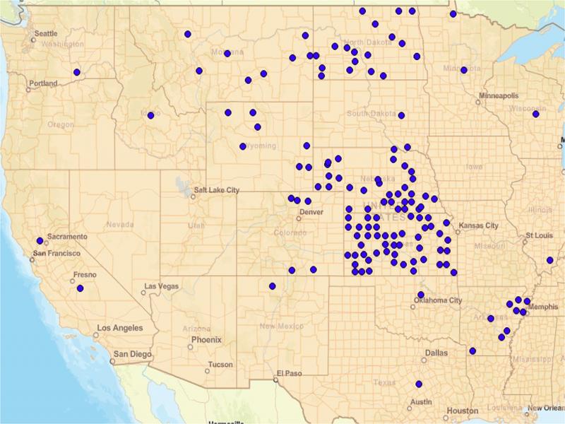
Figure 1:
Distribution of sampling sites by county for the Pratylenchus survey.
Table 1.
Number of fields sampled from states of the Great Plains region used in DNA barcoding study of Pratylenchus spp.
| States | Corn | Wheat | Dry beans | Potatoes | Barley | Alfalfa | Sugar beets | Total field | Field % |
|---|---|---|---|---|---|---|---|---|---|
| Nebraska | 97 | 8 | 0 | 5 | 0 | 0 | 0 | 110 | 44.72 |
| Kansas | 43 | 19 | 0 | 0 | 0 | 1 | 0 | 63 | 25.61 |
| Wyoming | 0 | 0 | 18 | 8 | 3 | 0 | 0 | 29 | 11.79 |
| North Dakota | 0 | 19 | 0 | 0 | 0 | 0 | 0 | 19 | 7.72 |
| Montana | 6 | 0 | 0 | 1 | 4 | 4 | 0 | 15 | 6.10 |
| Colorado | 5 | 0 | 0 | 2 | 0 | 1 | 2 | 10 | 4.07 |
| Total field | 151 | 46 | 18 | 16 | 7 | 6 | 2 | 246 | |
| Field % | 61.38 | 18.70 | 7.32 | 6.50 | 2.85 | 2.44 | 0.81 |
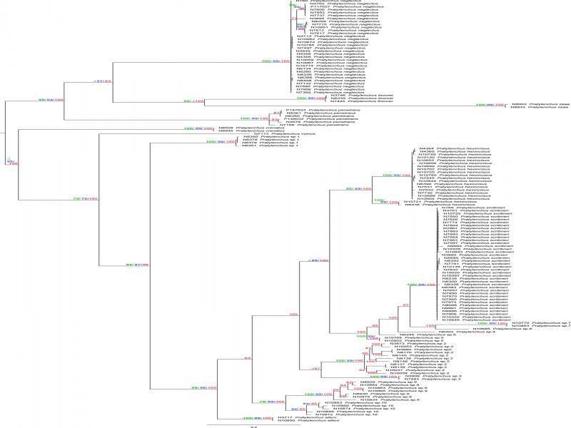
Figure 2:
Bayesian tree of unique COI haplotypes derived from 915 Pratylenchus specimen data set. Nodes are labeled according to tree building approach, with bootstrap values indicated in green for neighbor-joining, blue for maximum-likelihood, and red for posterior probability in Bayesian analysis. The absence of a value reflects the absence of that node, or bootstrap values below 50 in a particular tree building approach. Terminal nodes are labeled by Nematode Identification Numbers (NIDs) and taxon name.
Table 2.
Haplotype group representatives and their highest identity matches from GenBank as of August 29, 2019.
| Haplotype group (this study) | Blasted NID No. (this study) | COI Match Accession No. | Corresponding GenBank Name | Identity% | D2–D3 Match Accession No. | Corresponding GenBank Name | Identity% |
|---|---|---|---|---|---|---|---|
| P. neglectus | N10756 | KY424103 | P. neglectus | 99.8 | MG906766 | P. neglectus | 99.7 |
| P. penetrans | N6260 | KY816936 | P. penetrans | 99.8 | JX046986 | P. penetrans | 98.9 |
| P. thornei | N7566 | KY828316 | P. thornei | 99.5 | KYT213559 | P. thornei | 100 |
| P. alleni | N3717 | MK045330 | P. alleni | 99.3 | MN251270 | P. alleni | 100 |
| P. zeae | N8934 | KY424056 | P. zeae | 99.5 | |||
| P. crenatus | N8539 | KY816943 | P. crenatus | 100 | KY468865 | P. crenatus | 98.1 |
| P. vulnus | N7113 | GQ332425 | P. vulnus | 99.3 | |||
| P. scribneri | N7839 | MH016378 | P. scribneri | 99.5 | MK292133 KY828290 EU130841 |
P. scribneri
P. hexincisus
P. agilis | 99.7 99.7 99.7 |
| P. hexincisus | N7726 | MH016378 | P. scribneri | 81.0 | KX842632 EU130841 KY828291 |
P. scribneri
P. agilis P. hexincisus | 100 98.8 98.9 |
| Pratylenchus sp. 1 | N6350 | KU198944 | Pratylenchus sp. | 83.0 | MN251269 | Pratylenchus sp. | 99.6 |
| Pratylenchus sp. 2 | N8139 | MK045330 | P. alleni | 79.3 | MN251273 | Pratylenchus sp. | 100 |
| Pratylenchus sp. 3 | N3908 | MK045330 | P. alleni | 83.4 | |||
| Pratylenchus sp. 4 | N6402 | KY424092 | P. scribneri | 88.6 | |||
| Pratylenchus sp. 5 | N10767 | KY424092 | P. scribneri | 87.3 | MH730449 | P. scribneri | 99.2 |
| Pratylenchus sp. 6 | N6245 | KY424092 | P. scribneri | 88.5 | |||
| Pratylenchus sp. 7 | N10770 | KY424093 | P. scribneri | 85.2 | |||
| Pratylenchus sp. 8 | N10685 | KY424092 | P. scribneri | 89.1 | KT175531 | P. pseudocoffeae | 96.2 |
| Pratylenchus sp. 9 (1) | N10841 | KY424092 | P. scribneri | 80.1 | KT175531 | P. pseudocoffeae | 95.8 |
| Pratylenchus sp. 9 (2) | N8930 | KY424092 | P. scribneri | 79.7 | KT175531 | P. pseudocoffeae | 95.7 |
| Pratylenchus sp. 10 (1) | N10856 | MK045330 | P. alleni | 78.7 | |||
| Pratylenchus sp. 10 (2) | N10853 | MK045330 | P. alleni | 79.5 |
Table 3.
Estimates of evolutionary divergence (p-distances) over sequence pairs within (bold) and between groups.
| P. alleni | P. crenatus | P. hexincisus | P. neglectus | P. penetrans | P. scribneri | P. thornei | P. vulnus | P. zeae | ||
| P. alleni | 0 | |||||||||
| P. crenatus | 0.308 | 0.001 | ||||||||
| P. hexincisus | 0.216 | 0.355 | 0.022 | |||||||
| P. neglectus | 0.28 | 0.33 | 0.362 | 0.009 | ||||||
| P. penetrans | 0.322 | 0.348 | 0.399 | 0.298 | 0.038 | |||||
| P. scribneri | 0.172 | 0.327 | 0.199 | 0.317 | 0.351 | 0.003 | ||||
| P. thornei | 0.332 | 0.357 | 0.391 | 0.3 | 0.319 | 0.359 | 0 | |||
| P. vulnus | 0.235 | 0.328 | 0.321 | 0.317 | 0.325 | 0.29 | 0.33 | 0.007 | ||
| P. zeae | 0.33 | 0.377 | 0.399 | 0.334 | 0.354 | 0.367 | 0.329 | 0.348 | 0.002 | |
| sp. 1 | 0.209 | 0.3 | 0.283 | 0.304 | 0.332 | 0.231 | 0.326 | 0.263 | 0.327 | |
| sp. 2 | 0.228 | 0.357 | 0.222 | 0.373 | 0.396 | 0.232 | 0.389 | 0.342 | 0.409 | |
| sp. 3 | 0.182 | 0.352 | 0.231 | 0.324 | 0.357 | 0.189 | 0.359 | 0.291 | 0.344 | |
| sp. 4 | 0.174 | 0.316 | 0.207 | 0.316 | 0.331 | 0.118 | 0.348 | 0.274 | 0.356 | |
| sp. 5 | 0.195 | 0.33 | 0.181 | 0.334 | 0.352 | 0.125 | 0.359 | 0.302 | 0.361 | |
| sp. 6 | 0.187 | 0.334 | 0.197 | 0.315 | 0.358 | 0.108 | 0.354 | 0.296 | 0.364 | |
| sp. 7 | 0.171 | 0.299 | 0.212 | 0.3 | 0.333 | 0.153 | 0.327 | 0.256 | 0.341 | |
| sp. 8 | 0.165 | 0.308 | 0.221 | 0.299 | 0.345 | 0.12 | 0.327 | 0.278 | 0.359 | |
| sp. 9 | 0.202 | 0.33 | 0.244 | 0.338 | 0.353 | 0.206 | 0.347 | 0.265 | 0.361 | |
| sp. 10 | 0.195 | 0.342 | 0.214 | 0.35 | 0.35 | 0.211 | 0.351 | 0.262 | 0.372 | |
| sp. 1 | sp. 2 | sp. 3 | sp. 4 | sp. 5 | sp. 6 | sp. 7 | sp. 8 | sp. 9 | sp. 10 | |
| sp. 1 | 0.005 | |||||||||
| sp. 2 | 0.294 | 0.077 | ||||||||
| sp. 3 | 0.223 | 0.205 | 0.004 | |||||||
| sp. 4 | 0.219 | 0.233 | 0.186 | n/ca | ||||||
| sp. 5 | 0.253 | 0.209 | 0.199 | 0.132 | 0 | |||||
| sp. 6 | 0.236 | 0.223 | 0.191 | 0.112 | 0.079 | 0 | ||||
| sp. 7 | 0.199 | 0.235 | 0.185 | 0.16 | 0.163 | 0.159 | 0 | |||
| sp. 8 | 0.204 | 0.254 | 0.196 | 0.127 | 0.158 | 0.132 | 0.136 | 0 | ||
| sp. 9 | 0.237 | 0.246 | 0.221 | 0.2 | 0.201 | 0.202 | 0.207 | 0.206 | 0.048 | |
| sp. 10 | 0.25 | 0.212 | 0.226 | 0.207 | 0.208 | 0.21 | 0.216 | 0.213 | 0.156 | 0.034 |
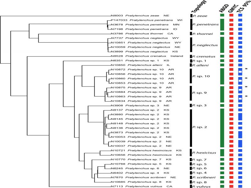
Figure 3:
Maximum likelihood tree of haplotype groups reflecting group membership support based on consensus tree topology, and species delimitation methods. These methods are indicated by colored bars: Automatic Barcoding Gap Discovery (ABGD) green bar, Generalized Mixed Yule Coalescent (GMYC) red bar, and statistical parsimony analysis (TCS) blue bar. TCS groups marked with an asterisk indicate a merging of two groups at a 90% connection limit.
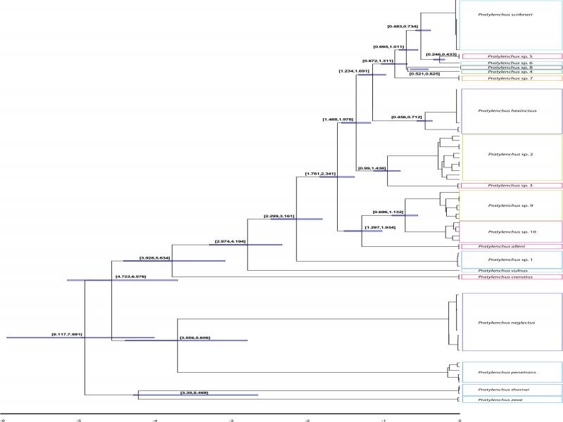
Figure 4:
Bayesian evolutionary analysis by sampling trees (BEAST) analysis of estimated divergence times using the mitochondrial substitution genome rate of 7.2 ×10⁻⁸ per site per generation, a calibration originally calculated for the nematode Caenorhabditis briggsae (Howe et al., 2010). The rate assumes two Pratylenchus generations per year. Divergence age confidence intervals of 95% are provided at nodes.
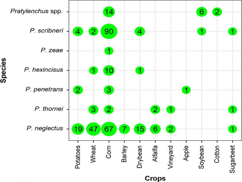
Figure 5:
Matrix exhibiting Pratylenchus species of the Great Plains and their host associations. The number of fields with a specific plant host-Pratylenchus species combination is indicated by the number within the green circles.
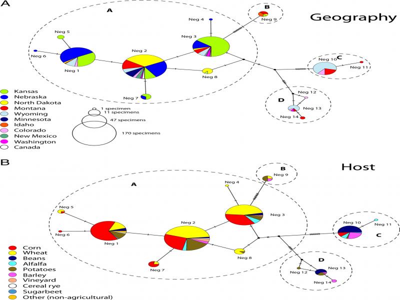
Figure 6:
TCS networks depicting Pratylenchus neglectus haplotype abundance and relationships among haplotypes. Dashed lines encircling haplotypes indicate 95% connection limits. Hash marks between haplotypes indicate number of mutational steps between haplotypes. Relative size of the circles reflects abundance of specimens exhibiting that specific haplotype. (A) Colors indicate geographic origin of the haplotypes in the Pratylenchus survey; (B) colors indicate the host in the field at time of the survey.
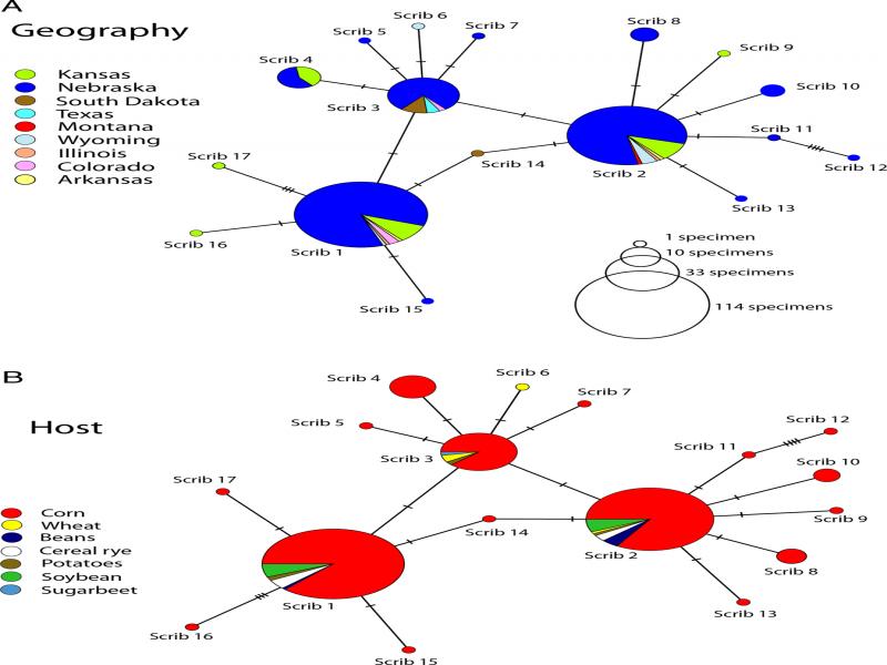
Figure 7:
TCS network at 95% connection limit depicting Pratylenchus scribneri haplotype abundance and relationships among haplotypes. Hash marks between haplotypes indicate number of mutational steps between haplotypes. Relative size of the circles reflects abundance of specimens exhibiting that specific haplotype. (A) Colors indicate geographic origin of the haplotypes in the Pratylenchus survey; (B) colors indicate the host in the field at time of the survey.
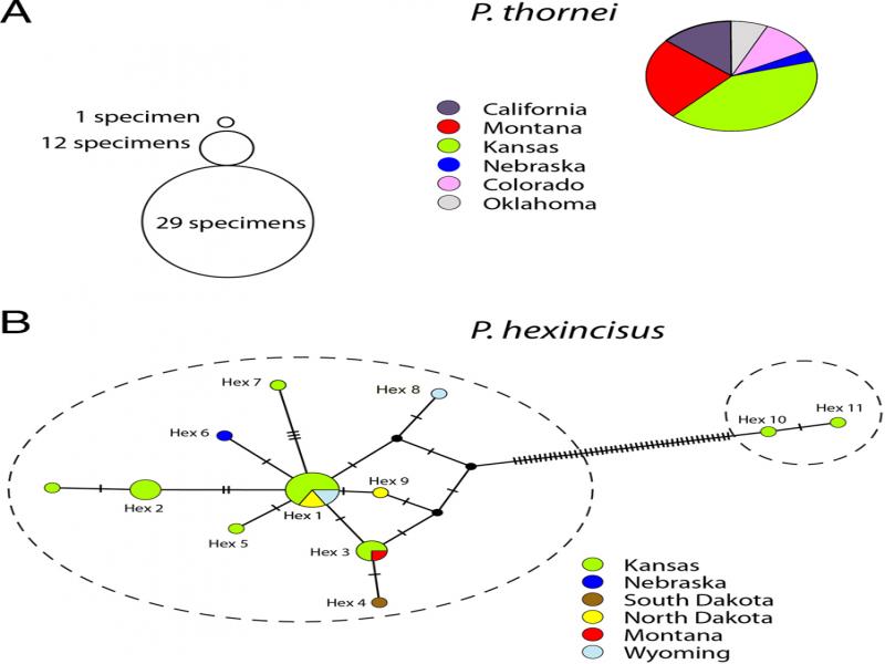
Figure 8:
TCS networks depicting (A) the single haplotype of Pratylenchus thornei and (B) the two networks exhibited by Pratylenchus hexincisus. Dashed lines encircling haplotypes indicate 95% connection limits. Hash marks between haplotypes indicate number of mutational steps between haplotypes. Relative size of the circles reflects abundance of specimens exhibiting that specific haplotype. Colors indicate geographic origin of the haplotypes in the Pratylenchus survey.
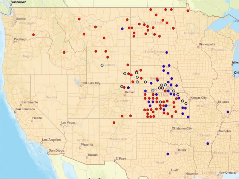
Figure 9:
County location of surveyed fields with Pratylenchus neglectus (red), P. scribneri (blue), and fields with a mixture of both species (gray).