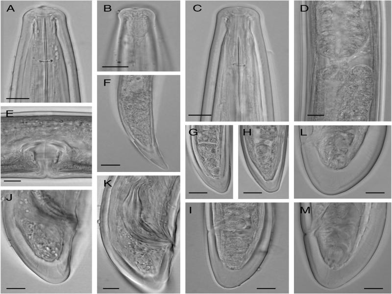
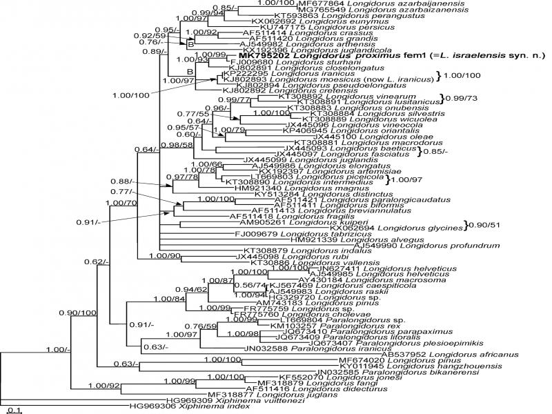
Longidorus proximus (Sturhan and Argo, 1983) was originally described as a parthenogenetic species. Later, a bisexual population was reported by Roca (1986). The species was reported from Iran in a conference abstract, but the morphological and morphometric data of this population were not available (Niknam et al., 2006).
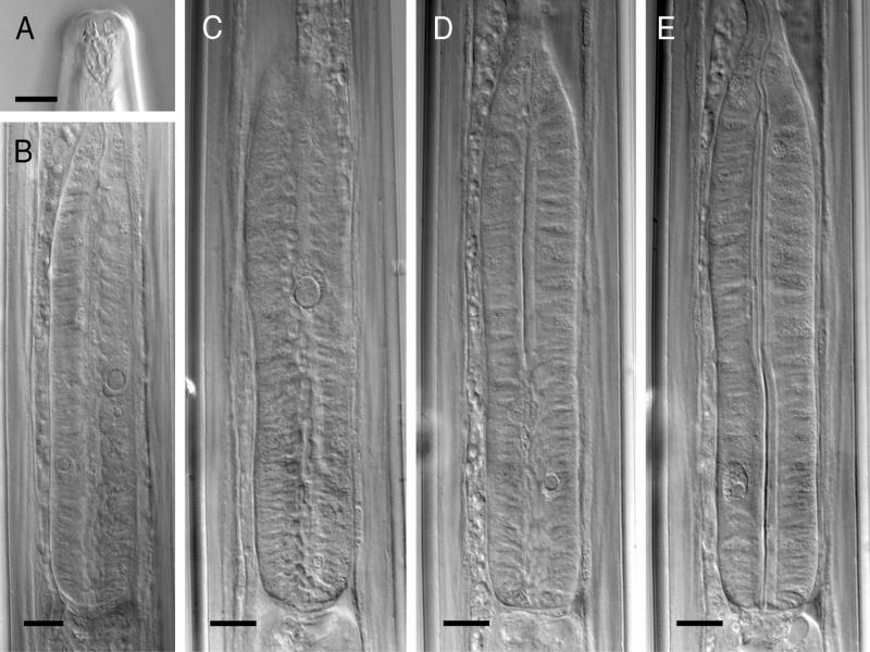
Longidorus israelensis (Peneva et al., 1998) is currently only known by its type population (Peneva et al., 1998) and has not been reported since its description. It was described on the basis of its morphological characteristics; the information on juvenile developmental stages, a tentative male, and molecular data were lacking. Recent studies (Zhao et al., 2017), however, emphasize using molecular data for reliable identification of cryptic species, especially for economically important and quarantine pests. The history of the reported Longidorus (Mikoletzky, 1922) species in Iran is given by Gharibzadeh et al. (2018). Some recent studies in Iran have focused on the molecular taxonomy of longidorids in Iran (Jahanshahi Afshar, 2019; Jahanshahi Afshar et al., 2019; Mirzaie Fouladvand et al., 2019; Mobasseri et al., 2019). During the present study, a population of Longidorus was recovered from a wheat-potato field in Hamadan province and was studied using morphological and molecular criteria. The recovered population looked similar to two species, L. proximus and L. israelensis, mainly by the shape of amphidial fovea and characteristics of the pharyngeal bulb, i.e., the arrangement and size of the glands nuclei. Thus, the present study aims to identify the recently recovered population of Longidorus and discuss on the taxonomy of L. israelensis.
Materials and methods
Sampling, nematode extraction, mounting, and morphological studies
A total number of 35 soil samples were collected from wheat and potato fields in the city of Hamadan during a survey to identify longidorid nematodes occurring in these fields. The soil samples were collected from 20 to 40 cm depth in May 2016. The longidorid nematodes were extracted by suspending the soil samples in water and collecting the specimens using 20 and 60-mesh (US standard mesh numbers, equal to 841 and 250-μm openings) sieves. The specimens studied here were recovered from a field with a wheat-potato rotation culture, hand-picked using a Nikon SMZ1000 stereomicroscope, heat-killed by adding boiling 4% formaldehyde solution, and transferred to anhydrous glycerin according to De Grisse (1969). Measurements were made using a drawing tube attached to an Olympus BX-41 light microscope. The juvenile stages were identified according to Robbins et al. (1995). The digital images were prepared using an Olympus DP72 digital camera attached to an Olympus BX51 microscope powered with differential interference contrast (DIC).
DNA extraction, PCR, and sequencing
For the molecular phylogenetic studies, two live nematode specimens were picked out, studied individually on temporary slides, photographed, and transferred to a small drop of TE buffer (10 mM Tris-Cl, 0.5 mM EDTA; pH 9.0, QIAGEN Inc., Valencia, CA) individually on separate clean slides, and each specimen was squashed using a clean slide cover glass. The suspension was collected by adding 50 μl TE buffer. Each sample was regarded as an independent DNA sample, and stored at −20°C until used as polymerase chain reaction (PCR) template. Primers used for the PCR amplification of the D2–D3 expansion domains of the LSU rDNA were forward D2A (5′-ACAAGTACCGTGAGGGAAAGTTG-3′) and reverse D3B (5′-TCGGAAGGAACCAGCTACTA-3′) (Nunn, 1992) primers. The internal transcribed spacer 1 (ITS1) fragment was amplified using the forward primer rDNA1 (5′-TTGATTACGTCCCTGCCCTTT-3′) and the reverse primer rDNA1.58s (5′-ACGAGCCGAGTGATCCACCG-3′) (Subbotin et al., 2000). PCR was carried out for both the aforementioned fragments in a total volume of 40 μl (12 μl distilled water, 20 μl 2x Master mix (Ampliqon, Denmark), 2 μl of each primer (10 pMol/μl), and 4 μl of DNA template). The thermal cycling program for both reactions was as follows: denaturation at 94°C for 5 min, followed by 32 cycles of denaturation at 94°C for 30 sec, annealing at 52°C for 40 sec, and extension at 72°C for 80 sec. A final extension was performed at 72°C for 10 min. The PCR products were purified and sequenced directly for both strands using the same primers with an ABI 3730XL sequencer (Bioneer Corporation, South Korea). The newly obtained sequences were submitted to the GenBank database under the accession numbers given in LSU and ITS1 trees.
Phylogenetic analyses
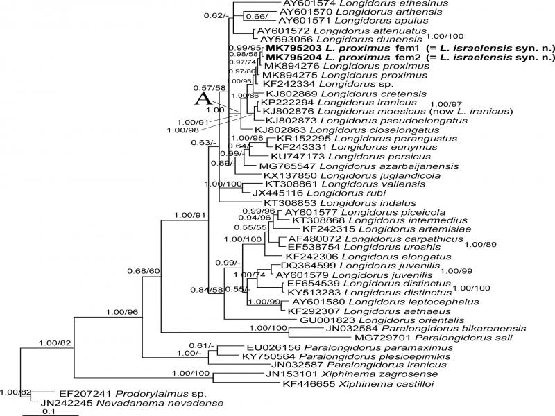
The newly generated sequences were compared with the available sequences in the GenBank database using the basic local alignment search tool (BLAST) (https:// blast.ncbi.nlm.nih.gov/Blast.cgi). For LSU phylogeny, several available sequences of the genus were retrieved from the database (a large and a smaller pruned LSU datasets were prepared). The currently available ITS1 sequences of Longidorus spp. were retrieved for the ITS1 phylogeny. The LSU sequences were aligned using ClustalX2 (www.clustal.org). The ITS1 dataset was aligned using MUSCLE as implemented in MEGA (Tamura et al., 2013), and the alignment of both datasets was edited using MEGA (Tamura et al., 2011). The appropriate model of base substitution was selected using MrModeltest 2 (Nylander, 2004). The Akaike-supported model, a general time-reversible model, including among-site rate heterogeneity and estimates of invariant sites (GTR+G+I), was selected and used in the phylogenetic analyses of both LSU and ITS1 datasets. Bayesian analyses were performed with MrBayes 3.1.2 (Ronquist and Huelsenbeck, 2003) by running the chains for five million generations for the three aforementioned analyses (the large and pruned LSU datasets, and the ITS1 dataset). After discarding burn-in samples and evaluating convergence, the remaining samples were retained for further analyses. The Markov chain Monte Carlo method within a Bayesian framework was used to estimate the posterior probabilities of the phylogenetic trees (Larget and Simon, 1999) using the 50% majority rule. For maximum likelihood (ML) analyses, raxmlGUI version 1.1 (Silvestro and Michalak, 2012) was used and the analyses were performed using the same model of nucleotide substitution in Bayesian inference (BI) (GTR+G+I) for the pruned LSU and ITS1 trees. For phylogenetic analyses of LSU dataset, Nevadanema nevadense (Álvarez-Ortega and Pena-Sañtiago, 2012) (JN242245) and Prodorylaimus sp. (EF207241) were used as outgroup taxa. Xiphinema index (Thorne and Allen, 1950) (HG969306) and X. vuittenezi (Luc et al., 1964) (HG969309) were used as the outgroup taxa in ITS1 tree. The output files of the used phylogenetic programs were visualized using Dendroscope V.3.2.8 (Huson and Scornavacca, 2012) and redrawn using CorelDRAW software version 13. The Bayesian posterior probability (BPP) and ML bootstrap (BS) values exceeding 50% are given on appropriate clades in the shape of BPP/ML BS.
Results and description
Iranian population of Longidorus proximus
= L. israelensis syn. n.
Measurements
See Table 1.
Table 1.
Morphometrics of Iranian population of Longidorus proximus (Sturhan & Argo, 1983).
| Stage/character | J1 | J2 | J3 | J4 | Female | Male |
|---|---|---|---|---|---|---|
| n | 1 | 3 | 12 | 4 | 19 | 1 |
| L | 1,792 | 2,197.3 ± 78.0 (2,125–2,280) | 3,141.7 ± 413.6 (2,540–3,892) | 4,762.8 ± 537.6 (4,395–5,547) | 6,728.4 ± 654.2 (5,600–8,570) | 9,167 |
| a | 69 | 73.2 ± 0.3 (72.9–73.5) | 85.9 ± 5.2 (75.8–93.7) | 109 ± 5 (101.7–112.7) | 111.6 ± 11.4 (96–142) | 143.2 |
| b | 72 | 6.7 ± 0.5 (6.1–7.1) | 9.2 ± 1.5 (7.5–12.1) | 10.9 ± 0.9 (10.2–12.2) | 13.8 ± 1.5 (11.6–17.0) | 203.7 |
| c | 37 | 50.8 ± 6.1 (43.7–54.5) | 71.7 ± 6.8 (62–84) | 114.3 ± 15.0 (102.2–135.3) | 166.2 ± 15.6 (141.8–191.0) | 191 |
| c' | 3 | 2.1 ± 0.2 (2.0–2.3) | 1.6 ± 0.1 (1.4–1.7) | 1.2 ± 0.1 (1.1–1.3) | 0.9 ± 0.1 (0.7–1.1) | 0.7 |
| V | – | – | – | – | 53.8 ± 2.9 (49.7–61.2) | – |
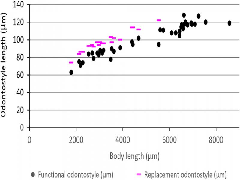
| Odontostyle | 67 | 74.0 ± 1.5 (72–76) | 78.8 ± 1.0 (82–84) | 100 ± 4 (96–104) | 117.5 ± 6.5 (108–127) | 119 |
| Replacement odontostyle | 77 | 94.5 ± 6.5 (89–101) | 94.5 ± 10.0 (92–111) | 113 ± 6 (105–118) | – | – |
| Odontophore | 24 | 38 ± 5 (33–44) | 36.5 ± 3.5 (33–40) | 47.5 ± 7.5 (36–52) | 60.5 ± 2.5 (58–64) | 66 |
| Total stylet | 91 | 112.5 ± 5.5 (108–119) | 119.5 ± 2.5 (117–122) | 146.5 ± 9.0 (135–156) | 178.0 ± 7.5 (169–189) | 175 |
| Width of lip region | 10 | 10.8 ± 1.6 (9–12) | 13.7 ± 0.7 (12.5–15.0) | 16.3 ± 1.0 (15–17) | 18.7 ± 1.0 (17–21) | 19 |
| Pharynx | 250 | 329.7 ± 28.6 (300–357) | 345.0 ± 29.7 (285–380) | 435 ± 28 (400–460) | 477 ± 21.3 (443–512) | 480 |
| Body width at mid-body | 26 | 30 ± 1 (29–31) | 36.7 ± 5.2 (30–47) | 43.8 ± 5.2 (39–50) | 61 ± 7 (50–75) | 64 |
| - at base of pharynx | 25 | 28 ± 0 (28–28) | 33.6 ± 3.1 (29–38) | 39.6 ± 2.1 (37–42) | 50.4 ± 4.4 (45–63) | 48 |
| - at anus level | 20 | 21.2 ± 1.0 (20–22) | 27.2 ± 2.4 (23–31) | 35.0 ± 1.8 (33–37) | 45.2 ± 3.8 (41–55) | 45 |
| - at guiding ring level | 15 | 16.7 ± 0.6 (16–17) | 19.9 ± 0.8 (19.0–21.5) | 23.1 ± 0.9 (22–24) | 27.1 ± 1.6 (25–32) | 28 |
| Anterior end to guiding ring | 18 | 22.7 ± 1.5 (21–24 ) | 25.8 ± 2.1 (23–29) | 29.3 ± 1.0 (28–30) | 35.4 ± 2.7 (31–40) | 36 |
| - to vulva | – | – | – | – | 3,619 ± 356 (2,900–4,590) | – |
| Tail length | 49 | 43.7 ± 5.7 (39–50) | 43.8 ± 3.7 (39–50) | 41.8 ± 1.0 (41–43) | 41.0 ± 3.3 (35–46) | 48 |