
Introduction
There has been extensive research and development regarding cancer in the medical field over last few decades. This need of development arises because of the fatality of the disease and hence early detection is key for providing proper treatment for the same. Cancer is an abnormal growth of cells concentrated to a particular part of the body with potential to spread extensively to other parts of the body making it one of the deadliest diseases in the world. The early stages of cancer are usually asymptomatic which makes it difficult to diagnose. Cancers like brain tumor are difficult to operate upon and require early detection. Treatment techniques need to be precise and accurate at every step of the way, especially while approaching the tumor, since it cannot be accessed physically. The very first step towards proper treatment and care is correct diagnosis. The right diagnosis paves the way towards finding the right solution and then implementing it. MRIs are the most popular diagnostic method for brain tumors. However, they are read manually and the tumor is identified and classified manually.
Existing detecting procedures like biopsy are invasive and involve the collection of tissue samples from the brain to check for abnormal cell growth and activity. They also involve manual labor and time. In recent years, Magnetic Resonance Imaging (MRI) has been preferred for its non-invasive properties. However, tumor segmentation using these MRI scans has been particularly challenging since it involves numerous processes to identify the tumor region from surrounding cerebral tissues and edemas.
The need is to develop a system that can reliably highlight the tumor-affected area and enhance existing testing procedures while being labour and cost efficient and keeping the patient’s health intact. Image processing has emerged as the leading contender in the world of brain tumor detection and segmentation. It has provided more accurate results as compared to the systems already in use. With a wider scope of expansion, it has the potential of being successfully adopted into regular clinical practice. This project attempts at developing a brain tumor detection tool that helps in the automation of brain tumor detection. The objective is to prepare an algorithm based on threshold segmentation and watershed algorithm that detects the tumor area in an MRI scan so that brain tumors can be diagnosed accurately and precisely with least possible manual intervention.
The article describes the execution of the proposed algorithm consisting of various procedures, and the subsequent research on the obtained output. The proposed algorithm accepts MRI scan as the input. A median filter is applied to the gray-scale image to filter out the noise. The image is then smoothed using a smoothing matrix in the form of an average filter. The top hat filter is used after smoothening to remove noise from the foreground of the image. This is followed by contrast enhancement to saturate the pixel intensity. The enhanced image then undergoes Image Binarization before undergoing morphological erosion to remove any excess pixels from the boundaries of the MR image. Morphological dilation adds pixels to fill in any gaps and holes within the image boundaries which may be caused due to presence of noise, thus increasing the quality of the image.
The threshold algorithm is now executed. In this, a threshold value is calculated and set based on the average of intensity values of each pixel in the image. The image obtained is then used for watershed segmentation. K-means clustering is executed after watershed segmentation, followed by MSER detection. The detected tumor region is obtained and highlighted in the final output.
Finally, a performance evaluation of the proposed method is carried out based on several parameters such as Structural Similarity Index Measure (SSIM), Feature Similarity Index Measure (FSIM) and Peak Signal-to-Noise Ratio (PSNR). The values obtained provide an insight on the image quality enhancement capabilities of the mentioned methodology. Further, to verify the results obtained, the proposed algorithm is compared with two other existing algorithms, which very mainly in pre and post processing techniques used. This comparison draws light to the significance of choosing an appropriate combination of pre and post processing techniques and their impact on the results.
Literature review
Lu et al. (2019) perform morphological filtering as a pre-processing technique followed by watershed segmentation. However, this process yields inaccurate edge locations due to minimal noise filtering by the pre-processing techniques.
Hasan and Ahmad (2018) devise an algorithm with preprocessing techniques such as trilateral filter and then a median filter. The preprocessed image from here is used for watershed segmentation. The authors suggest that pre-processing techniques can be used to overcome the disadvantage of over segmentation by watershed algorithm by minimizing detailed texture of the image through smoothening.
Apart from this, these techniques can be beneficial in noise removal with the help of median filter, image sharpening using gaussian high pass filter and contrast improvement. Sivakumar and Janakiraman (2020) propose the use of edge detection using Enhanced Canny Edge Detection (ECED) to maximize the accuracy of segmentation process. Further, they also use a high pass filter as a prerequisite to the Enhanced Canny Edge Detector. They use a modified watershed segmentation in an attempt to improve the accuracy and sensitivity.
Dhage et al. (2015) propose a method that uses a median filter as the first step of preprocessing. This is followed by watershed segmentation along with Connected Component Labelling (CCL) to detect tumor regions. They also include numerous parameter calculations to check functionality of the algorithm such as Mean Square Error (MSE), PSNR, correlation and contrast parameter.
In the above-mentioned papers, it can be observed that they only employ watershed segmentation along with a few pre-processing techniques. Watershed algorithm paired with threshold segmentation makes the separation of tumor easier and makes the system faster. It gives precise positioning of the tumor and provides accurate regional boundaries. However, this combination has disadvantages like over segmentation and high sensitivity to detailed textures in the image which can be solved by using one or more pre-processing algorithms in combination with various post-processing techniques to enhance performance.
The literature mentioned before employs pre-processing techniques along with watershed segmentation. While tumor detection using watershed algorithm does not necessarily need post-processing, the use of certain techniques can help in image enhancement and provide better visual representation of the identified tumor region.
Morphological filtering helps in accurately segmenting the MRI by noise and magnetic field. The papers mentioned below highlight the advantages of including post processing techniques.
Tarhini and Shbib (2020) suggest that MRI scans are preferred over CT scans for tumor detection because MRI scan can create a much more detailed image of the body part and is more adapted to capturing small or hard to detect tumors when compared to CT scans. There has been extensive research based on various ways of incorporating different types of technologies for creating automated systems that can accurately spot brain tumors at the earliest. Their proposed system performs threshold segmentation followed by watershed segmentation to highlight the tumor region. Morphological operators are then used to increase the image quality as part of the post processing.
These systems are based on several techniques such as deep learning, machine learning, Convoluted Neural Networks (CNN) and image processing (Cui et al., 2009; Hore and Ziou, 2010; Mason et al., 2019).
Khan et al. (2019) perform a gamma contrast stretching using a Gaussian filter. Tumor extraction is carried out using Watershed segmentation proceeded by post processes such as Maximally Stable Extremal Region (MSER) and Histogram Oriented Gradients (HOG) that are used for feature extraction and removal of irrelevant features observed after watershed segmentation. Chi-square distance is calculated for feature selection.
Seere and Karibasappa (2020) use a combination of contrast enhancement, median filter and stationary wavelet mechanism to pre-process the image. They then perform segmentation in two phases—the first involving threshold segmentation and the second being watershed segmentation to group pixels of similar intensities together. They also mention the use of a supervised machine-learning algorithm, Support Vector Machine (SVM), to classify tumors post segmentation.
Shahin (2018) proposes a fast algorithm to detect the tumor region. The pre-processes used are sobel detector to obtain gradient of the input image. It is followed by skull-stripping technique to remove the skull area from the image. Subsequently, watershed segmentation is performed on the image. The paper classifies the features of segmented areas into three types—geometric, texture and gradient as part of its post processing techniques in order to study and analyse the segmented area. The final post process used is the Top-hat filter for reducing the brightness of the image.
Jemimma and Vetharaj (2018) focus on Dynamic Angle Projection Pattern (DAPP) as a post-processing method after watershed segmentation. This method uses a 5×5 mask where the pixel value at the middle is rotated 45° with respect to the neighboring pixels. This masked image is convoluted with the image from watershed segmentation and binarization of the pixel intensity is done. The values are encoded in decimals and the intensity can now be read in terms of texture. At the end, tumor classification is done using Convolutional Neural Network (CNN) using two layers namely, the pooling layer and the convolution layer.
Mustaqeem et al. (2012) aim to detect the tumor region by pre-processing the image using median filter in combination with a Gaussian high pass filter to sharpen the image. They then perform threshold segmentation followed by watershed segmentation to highlight the tumor region. Morphological operations like erosion and dilation are used as post-processing techniques which provide a final image with a highlighted tumor region.
Oo and Khaing (2014) use a balance of preprocessing and post processing to obtain an efficient method. They start by filtering the image to remove noise and performing skull stripping, making it easier to point out the tumor region. This is followed by watershed segmentation, while morphological erosion is done as a post-processing method. This method removes the surrounding tissue of the tumor region, drawing attention to the desired section of the brain. It also displays the area of the tumor region detected.
S. Sabarinathan, Dr. M. Poonguzhali, M. Pradeepkumar, S. Indhumalini, R. S. Kamalakannan (Bahadure et al., 2017) present a system which initially converts an image into its greyscale equivalent. A median filter is then used to enhance image quality by reducing the noise. This pre-processing technique is followed by watershed segmentation to identify and locate the tumor area and highlight the edges of the tumor. As part of their post processing, the paper employs morphological operations, giving a clear output image (Pambrun and Noumeir, 2015; Zhang et al., 2011; Zhao et al., 2006).
A proper combination of pre-processing and post-processing techniques along with watershed algorithm and threshold segmentation can provide a highly accurate and reliable system to detect brain tumor from MRI scan which has high computation speed and low complexity. The system obtained can be evaluated on and compared with other similar algorithms based on various statistical parameters such as Normalized Absolute Error (NAE), SSIM, and PSNR to give standardized results.
Proposed methodology
The pre-processing techniques are aimed at enhancing the image by filtering the noise, adjusting the contrast, smoothening, eroding and dilating the image. This helps thresholding and watershed segmentation by providing an easily detectable tumor region from the image and overcoming the major disadvantages of these two processes. Post-processing techniques like k-means clustering and Maximally Stable Extremal Regions (MSER) further enhance the detected tumor region and highlight it, making it easy to read and understand (Figure 1).
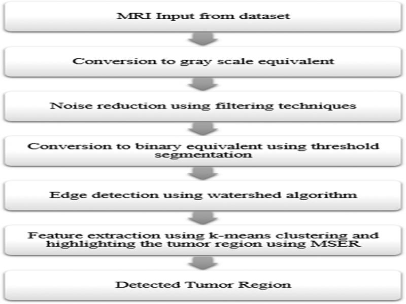
Figure 1:
Proposed methodology.
Pre-processing stage
The MRI scan is taken as the input. The primary aim of this stage is to reduce the amount of noise and disturbance in the image to make the subsequent processing easier.
Gray-scale conversion: The color-scheme of the image is checked and the image is converted to greyscale if it is in any other color-scheme.
Median filter: A median filter is applied which takes nine pixels at a time and fixes the median value of all nine as the output intensity, filtering the noise (Figure 2).
Image smoothening: The image is then smoothened using a 2 × 7 smoothening matrix consisting an entire row of 1s and zeros. This matrix functions as the operating window of the smoothening filter as it advances window by window for averaging-out pixel values. The 1s are used for entering pixel values in the matrix without manipulating them, since values are entered as sum of products. The 0s provide a zero padded input, which makes the matrix compatible to the subsequent smoothening function.
Top-hat filter: The top hat filter removes noise from the foreground of the image. It does so by extracting small elements and details from the image (Figure 3).
Contrast enhancement: Contrast is enhanced by saturating the top 1% and bottom 1% of the intensity values (Sara et al., 2019).
Image binarization: This is carried out to convert the entire image into a matrix of 1s and 0s depending on the intensity value. The output thus obtained is a black and white image.
Morphological operations: Morphological erosion removes any excess pixels from the boundaries of various regions while morphological dilation adds pixels to fill in any gaps and holes within the boundaries (Figure 4).
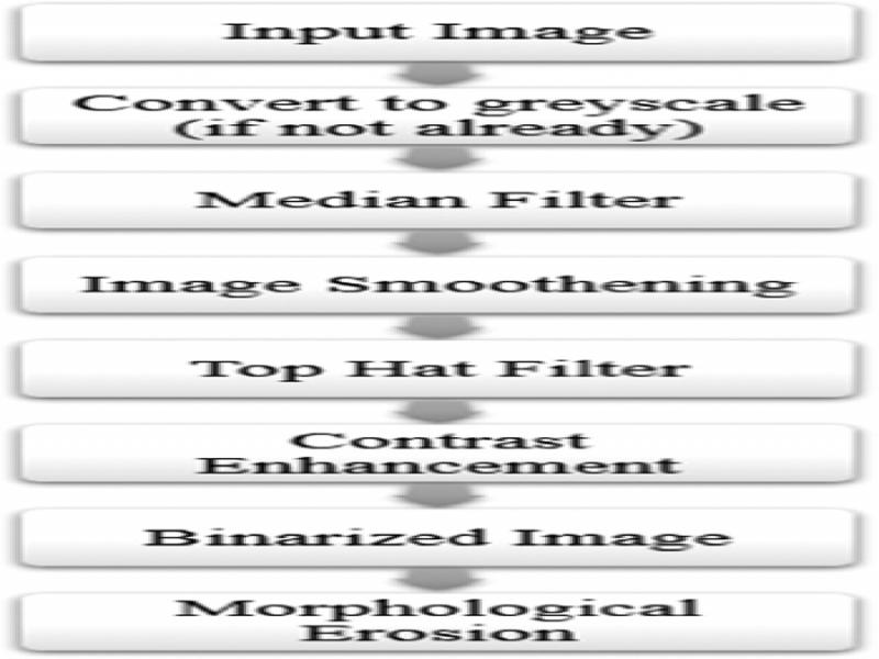
Figure 2:
Pre-processing techniques.
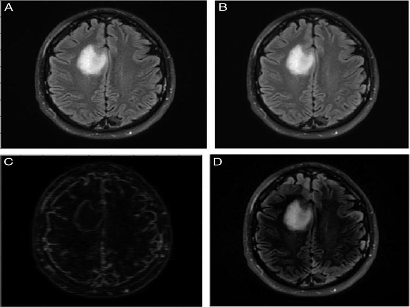
Figure 3:
Pre-processing phase 1. (A) Grayscale image, (B) Image after median filter, (C) Image after smoothening, (D) Image after top-hat filter.
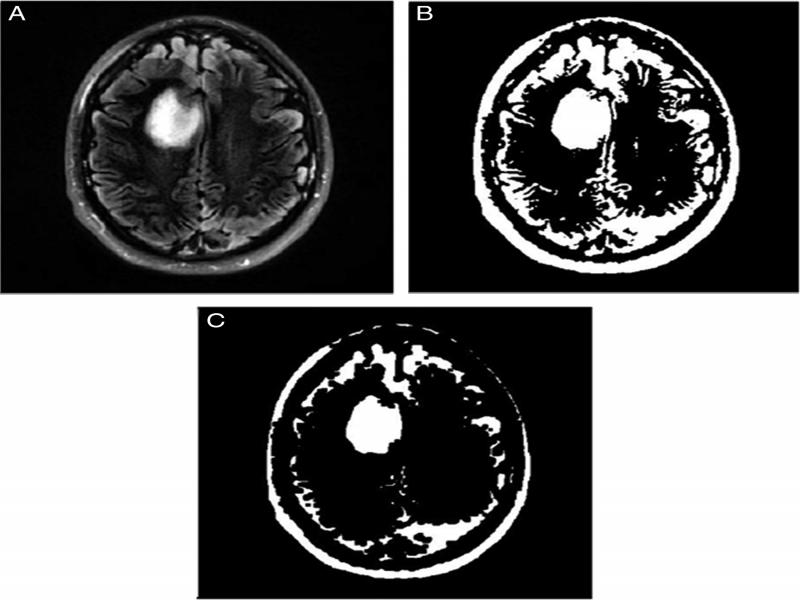
Figure 4:
Pre-processing phase 2. (A) Contrast enhancement, (B) Image after binarization, (C) Image after morphological erosion.
Processing stage
Thresholding: The threshold algorithm is now executed. In this, a threshold value based on the average of all intensity values is set. Pixel intensities more than the threshold value are set as one and the ones less than the threshold value are set as zero.
Watershed segmentation: The image obtained after threshold algorithm is complemented before being used for watershed segmentation. Complementing the image involves conversion of 0s in the threshold matrix to 1s and vice versa. In watershed segmentation, the entire image matrix is viewed as the watershed area where the image region is the catchment basin and the edges of image objects are the ridgelines. The brighter the pixel, the higher it is in the catchment region. The local maximas obtained using watershed segmentation are region based and the pixel intensities are grouped accordingly (Sara et al., 2019) (Figures 5 and 6).
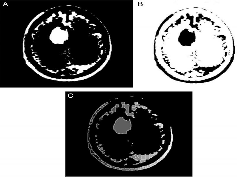
Figure 5:
Processing (A) Thresholding, (B) Complement of image, (C) Image after watershed segmentation.
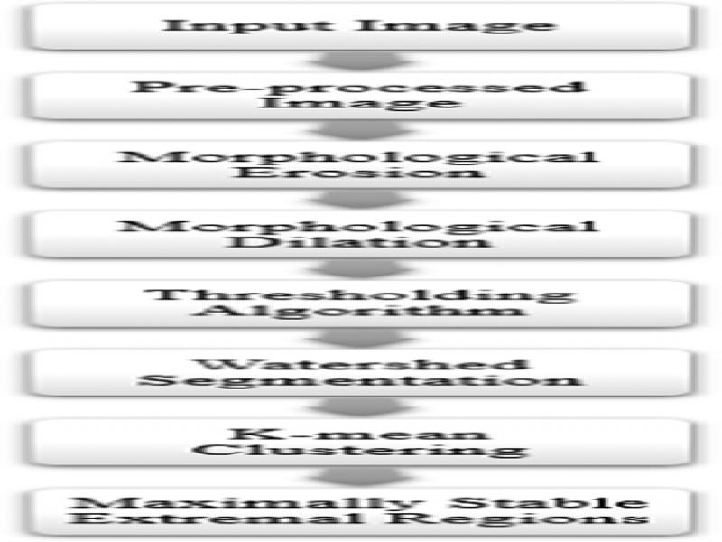
Figure 6:
Processing and post-processing techniques.
Post-processing stage
The segmented image is then subjected to post-processing techniques.
The two post-processing techniques used in the proposed methodology include k-means clustering and Maximally Stable Extremal Regions (MSER).
K-mean clustering: In k-mean clustering, the image is segmented into ‘k’ different clusters. For this procedure, the value of k is taken as 4. ‘K’ centroids are set and the clustering is done based on the least distance of a pixel from the centroid. These centroids are processed one at a time and result in the formation of 4 layers of the image containing different pixel groups. These four layers, when superimposed make the entire image.
Maximally stable extremal regions (MSER): MSER function fine-tunes the similar intensity pixels by grouping them according to intensity bands. This method is used for blob detection and connects areas of similar intensity. Thus, the detected tumor region is obtained and highlighted for better visualization (Figure 7).
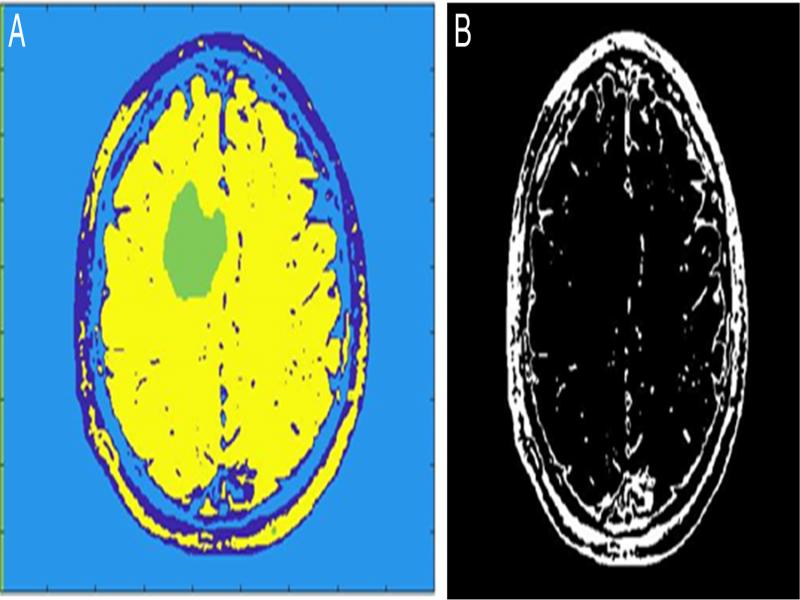
Figure 7:
Post-processing (A) Image with four different coloured clusters superimposed after K-Means clustering and (B) Image after MSER detection.
Experimental outcome
The outcome of the proposed methodology is seen in figure 9. Figure 8 represents the input image and figure 9 is the processed image with the highlighted tumor region.
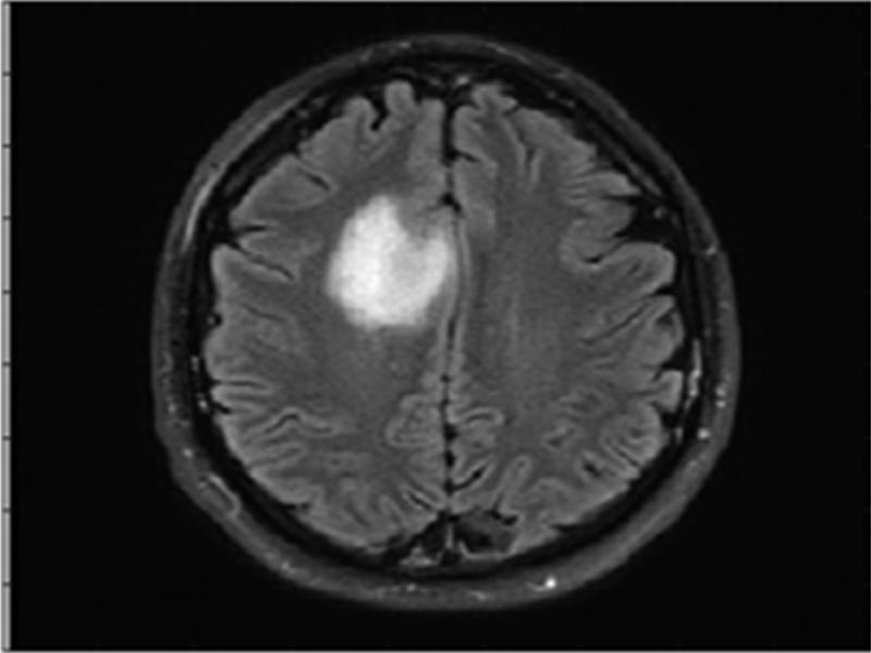
Figure 8:
Input image.
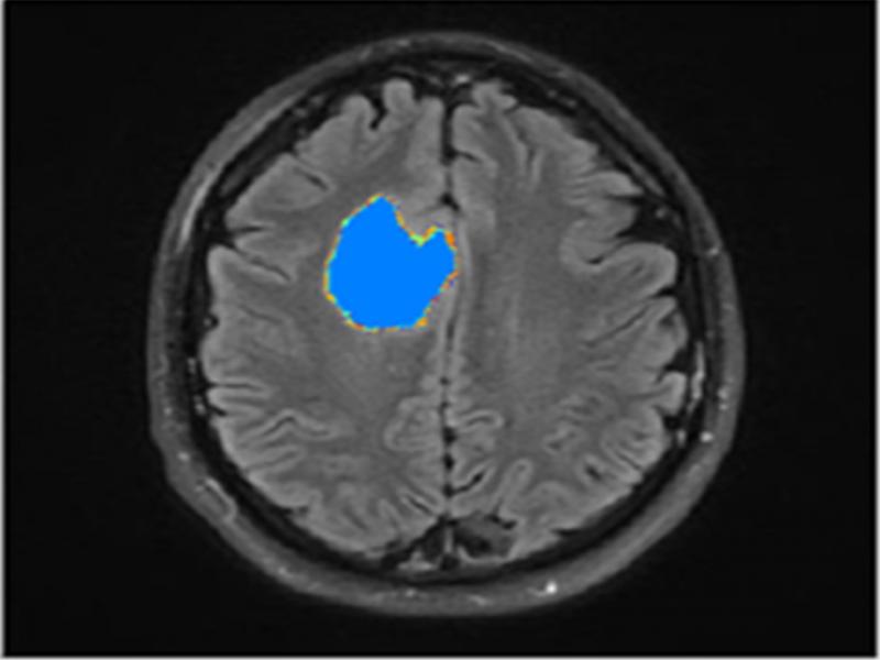
Figure 9:
Output image.
A distinct highlighted tumor region is visible in the final output image.
Performance evaluation metrics
A set of images was selected and evaluated on six parameters, namely, PSNR, Structural Similarity Index Measure (SSIM), FSIM, Entropy, Normalized Absolute Error (NAE) and Normalized Cross Correlation (NCC).
PSNR: It is the ratio of power of the signal to the power of noise to distort the signal.
The more the value of PSNR, the less is the noise causing distortion. It uses two parameters: range of image datatype and the mean square error between the input and reference image.
SSIM: It is a normalized measure used to find the similarity between input and processed image. Comparison parameters are luminance, contrast and structure:
where, ‘µ’ is the luminance, ‘σ’ is the contrast and C1, C2 are the constants for stability.SSIM quantifies degradation caused by pre-processes in an image. The function looks for similarities in pixel densities in the processed, reference image, and groups them.
FSIM: It is similar to SSIM except that the comparison parameters are phase congruency and gradient magnitude and that the minor features are compared:
where ‘SPC’ and ‘SG’ are the similarities based on phase congruency (PC) and gradient magnitude (GM), while α and β are parameters used to adjust the relative importance of PC and GM features.FSIM is used to measure the quality of image. Features of the two images are compared based on light intensity variations and change in intensity in a given direction.
Entropy: It is the quantification of the amount of information that an image contains. Entropy and information are directly proportional.
where X denotes the image to be quantified, xi denotes level i, p (xi) denotes probability of level i, b denotes units (as image pixel is coded in bits, b = 2) and n denotes the number of levels.Entropy quantifies the texture of the image, thus indicating the amount of information carried by the image. It translates the value of pixel intensity in terms of a numerical parameter width.
NAE: It is the measure of difference between original and processed image. It denotes the numerical variance between the two images:
where A and B are the image pixel values of the reference image and processed image respectively for a given dimension of m × n.NAE measures the exact difference between the processed and reference image.
NCC: Normalized Cross Correlation (NCC) is a parameter used for template matching. It is used to find instances in the processed image that match the original image:
where A and B are the image pixel values of reference image and processed image, respectively, with dimension (m × n).NCC quantifies closeness between two images. It goes window by window in the reference and processed image to calculate cross correlation values.
Discussion
A set of images was selected as a dataset and their evaluation parameters were calculated. A small subset of the obtained data is presented below (Table 1).
Table 1.
Statistical analysis.
| Parameter | ||||||
|---|---|---|---|---|---|---|
| Image | PSNR | SSIM | FISM | Entropy | NAE | NCC |
| Image 1 | 14.548 | 0.709 | 0.961 | 6.275 | 0.449 | 0.875 |
| Image 2 | 14.694 | 0.659 | 0.939 | 6.033 | 0.501 | 0.804 |
| Image 3 | 18.021 | 0.612 | 0.88 | 5.301 | 0.436 | 0.855 |
| Image 4 | 14.26 | 0.725 | 0.8666 | 6.159 | 0.463 | 0.775 |
| Image 5 | 15.775 | 0.708 | 0.881 | 4.8 | 0.618 | 0.712 |
| Image 6 | 19.624 | 0.809 | 0.876 | 5.337 | 0.288 | 0.906 |
| Image 7 | 18.961 | 0.748 | 0.941 | 6.376 | 0.3 | 0.948 |
| Image 8 | 29.673 | 0.934 | 0.96 | 4.473 | 0.08 | 0.991 |
| Image 9 | 19.89 | 0.886 | 0.939 | 6.51 | 0.271 | 0.931 |
| Image 10 | 17.931 | 0.806 | 0.937 | 6.493 | 0.344 | 0.846 |
| Different approaches | |||
|---|---|---|---|
| Parameters | Proposed algorithm | (Tarhini and Reda, 2020) | (Oo and Aung Soe, 2014) |
| PSNR | 18.4537 | 9.73795 | 18.97545 |
| SSIM | 0.79545 | 0.1833 | 0.29315 |
| FSIM | 0.92583 | 0.4439 | 0.75115 |
| Entropy | 5.8122 | 0.91185 | 4.8462 |
| NAE | 0.368 | 0.9941 | 0.28255 |
| NCC | 0.8801 | 0.37585 | 0.9122 |