Introduction
Nowadays, people are very talkative on the web. Due to the exponential growth in user feedback data, it becomes necessary for every product or service to do the mining of this feedback. Web opinion data are one of the main influential factors for purchasing products or services online. Web opinion data were the primary factor in decision-making during the last year when movements are restricted due to pandemic situations. To get the in-depth inside, the web opinion data aspect-based sentiment analysis (ABSA) has gained much attention in the last decade, and it continues a thrust area of research. Various studies have shown the effectiveness of recurrent neural network-based models for the sentiment classification task in the recent past. Different hybrid models are proposed, which use convolution neural network (CNN) and LSTM for the classification task.
Now the research question/direction that comes out is to propose an efficient deep neural network model for the sentiment classification task. So this work focuses on topic modeling and recurrent neural network-based approaches for ABSA. We have chosen LDA (Latent Dirichlet allocation), the most popular unsupervised topic model, and LSTM recurrent neural network. LDA is extensively used for unsupervised topic mining, and LSTM able to handle long-term dependencies. Following are the contribution of this paper:
A hybrid model based on topic modeling and recurrent neural network is proposed for sentiment analysis.
An efficient multi-layer Bi-LSTM is proposed for sentiment classification with only two stacked layers for keeping the model less complicated.
A hill climbing-based approach is proposed for tunning the hyper-parameter model to improve the proposed model’s accuracy. Pre-trained embeddings like Glove is used to improve efficiency.
A comparative analysis using multiple datasets is presented, demonstrating the performance improvement of the proposed approach.
The main objective of this work is to present an efficient hybrid model for sentiment classification using topic modeling and recurrent neural network. Model hyperparameters are tunned using an incremental approach, and pre-trained embeddings are also used for further performance improvement. The novelty of the proposed work is its efficiency with less complexity.
The paper’s remaining sections are as follows: the second section sheds light on the field’s most recent work. The background and intuition of LDA, Bi-LSTM, and pre-trained embedding are provided in the third section. In the fourth section, the methodology and proposed algorithms are explained. Experimental details with results are described in the fifth section. With a summary and future direction, the sixth section concludes the paper.
Related work
Sentiment analysis has got very much attention for more than one decade. Recently deep neural network-based approaches have gained popularity. Various hybrid models are presented using RNN, CRF, and topic modeling. This section discusses recent work done in the field of sentiment analysis of text reviews. Mainly LDA and RNN-based latest approaches are discussed along with their hybrid models.
Hameed et al. discuss a deep neural network-based model for sentiment classification with a single Bi-LSTM layer (Hameed and Garcia-Zapirain, 2020). Minaee et al. (2019) presented an ensemble approach based on LSTM and CNN for sentiment analysis with Glove pre-trained embedding. Rhanoui et al. (2019a) proposed an integrated CNN and Bi-LSTM model for document-level sentiment analysis with pre-trained Doc2vec embedding.
A deep neural network model approximates LDA to speed up the inference time (Zhang, D. et al., 2016). A novel approach is proposed using the CNN model with general-purpose embeddings and domain-specific embeddings of pre-trained embeddings for aspect extraction (Xu et al., 2018). A cosine similarity and Jensen–Shannon divergence are used to compute the similarity among topics and associate them into an aggregated model. The model is generated by the latent Dirichlet allocation and non-negative matrix factorization (Blair et al., 2020).
Bi-LSTM is used to analyze reviews through statistical analysis and sentiment classification (Huang et al., 2018a). The LSTM attention model for aspect-level sentiment analysis is proposed using embedding and common sense knowledge. An attention-based LSTM model is used for word sequence in a given document with a latent topic modeling layer. A tree-structured LSTM generates a semantic representation of the text (Zhang, W. et al., 2019).
A hybrid model based on LDA and LSTM has been given for COVID tweet analysis (Jelodar et al., 2020). The authors introduced LSTM based two models for aspect-based sentiment analysis (Huang et al., 2018b). One CRF-based character level model is for opinion target extraction, and the second attention-based sentence level model for classifying sentiment polarity.
A recommendation system using the topic model and DNN for the crowdfunding platform was developed (Shafqat and Byun, 2019). Two Bi-LSTM-based model in combination with 2D-Poling and 2D-CNN is given for sentiment analysis task (Zhou et al., 2016). A semantic similarity-based hybrid LDA model with LSTM is used for sentiment analysis of hotel reviews (Priyantina and Sarno, 2019). A hybrid approach was proposed (Luo, 2019) for sentiment analysis based on LDA and GRU-CNN. LDA is used for feature vector construction, and CNN with GRU is used for sentiment classification. A framework used topic modeling for finding rare named entities from text. This hybrid approach used LDA, LSTM, and CRF in an integrated way (Jansson and Liu, 2017). A CNN-Bi-LSTM-based hybrid model for document-level sentiment analysis is combined with the Doc2vec embeddings to improve the performance (Rhanoui et al., 2019b).
For short-text classification, an LSTM-based model is presented with Word2Vec (Wang et al., 2018). A model with a bidirectional recurrent neural network (RNN) with LSTM is implemented for recommendation and sentiment classification (Agarap and Grafilon, 2018). Pre-trained embeddings are used for training contextual semantics. A mortality prediction model was implemented from ICU admitted patient’s clinical remarks using LDA and LSTM with simultaneous training and learning (Jo et al., 2017). A recurrent structure is applied for contextual information with a max-pooling layer that analyses suitable words for text classification to capture the key components in texts (Lai et al., 2015).
Coronavirus (COVID-19)-based tweets are analyzed with NLP and sentiment classification using RNN (Nemes and Kiss, 2021). Tweet classification is done based on coronavirus using ML-based Naïve Bayes method (Jim et al., 2020) and ML with LDA (Xue et al., 2020). The author proposed a Gaussian membership function implementation based on a fuzzy rule base to analyze sentiments from tweets on COVID-19 (Chakraborty et al., 2020). An AI-based method is used for COID-19 sentiments (Man et al., 2020).
The performance of the LSTM model significantly depends on the value of its hyperparameter. There is no well-defined rule for selecting the values of hyperparameters. Yadav et al. (2020) presented an incremental approach for tuning LSTM hyperparameters.
From the above study, it is observed that most of the models are developed using multi-layer Bi-LSTM and CNN. Some of the models use hybrid or ensemble models. This study proposes a research direction to develop an efficient hybrid model for the sentiment classification task with optimization of various model hyperparameters. A new model can be designed, which may give better accuracy with comparatively less complexity.
Background
Latent Dirichlet allocation (LDA)
Topic modeling is an unsupervised NLP technique representing a group of text documents with several topics that can best explain each document’s underlying information. LDA primarily assumes that each document is a mixture of topics, and each word has a certain probability of falling into a particular topic (https://www.kaggle.com/rahulin05/sentiment-labelled-sentences-data-set). In LDA, every word in every document comes from a topic. The topic selects from a per document distribution over topics. The topic distribution ϴ for every document is proportional to Dirichlet (α), and the word distribution Ф is proportional to Dirichlet (β). Hyperparameters α and β have a vital role in the generative process of LDA. Parameter α controls the documents topic concentration means. The small value of α represents the documents as a mixture of a few topics, whereas its high value results in more topics per document. Similarly, parameter β controls topic word concentration. A low value of β represents the topics with fewer unique words making it more distinct, and its high value results in more unique words in each topic.
The topic generation process of LDA depends on the following two probability distributions:
= The probability distribution of topics in documents ϴtd.
= The probability distribution of words in topics Фwt.
The utmost goal of LDA is to estimate the probability of a word given document, i.e. , with the help of the above two mentioned probabilities, which is provided by:
It is the dot product of ϴtd and Фwt for each topic t where:
Gibbs sampling is applied for successively sampling conditional distributions of variables. In the long run, distribution over states converges to the accurate one. The equation for the same is below:
(2)where nd.k is the # document d use topic k; vk,w is the # topic k uses the given word; and α and β are the Dirichlet parameter for the document to topic and topic to word distribution, respectively (Blei et al., 2003).Long short-term memory (LSTM)
Cell-state and multiple gates are LSTM’s central concepts. Cell-state transmits relative data through the succession chain. It is just like to network’s memory. Important information retains in the cell state during sequence processing. To minimize the lack of memory effects, data coming from the previous time step leads to the next steps. The cell state moves when data are going to be added or removed via gates to that state. The gates are various neural networks that evaluate activated cell state data. Gate learns which data are necessary to keep or forget in the duration of training (http://colah.github.io/posts/2015-08-Understanding-LSTMs/).
Forget gate
The first gate is called the ‘forget gate’, which determines what data to store and discard. Present state input and hidden state information pass via the sigmoid function that returns the values from 0 to 1. If the value is around 0, discard it, and if the value near 1, then store it.
Input gate
The cell state changes through the gate. Next, the current input and the previous hidden state is transfer into a sigmoid function. We also convert current input and hidden state into the tanh function to squash the values from ‒1 to 1. Now multiply sigmoid output with tanh output. The sigmoid output specifies the retention of the needed information from the tanh output.
Cell state
There is now ample information for cell state calculation. In the first case, multiply the cell state with the forgot vector. If values compound it close to 0, the cell state decreases the values. We then take the input gate’s output and apply a point-wise addition to change the cell state to new values that the neural network can accept. This process gives a new cell state.
Output gate
The last gate is named as output gate that defines the condition next hidden state. The hidden state contains previous input information and is used to predict future value. The hidden state and new input are then given to a sigmoid function. Then we transfer to the tanh feature the newly changed cell status. We raise the tanh output with the sigmoid output to determine which data will be in the hidden state. The new cell state and the hidden state will shift to the next level.
The equations for the gates in LSTM are:
(3) (4)where sigmoid function is σ; weight for the respective gate neuron (x) = wx; so wi, wo, and wf are the weight of input, output, and forget gate neuron; the output of the previous hidden state is at time t‒1 is ht‒1; current state input, i.e., at time-stamp t, is xt; biases for the respective gates is bx; so bi, bo and bf are the biases of input, output, and forget gate.
Candidate for cell state at timet:
Cell state at time t is:
(7)Bi-directional LSTM
A bidirectional LSTM or Bi-LSTM consists of two LSTMs: one heading in a forward direction and the other backward. It is a sequence processing model. BiLSTMs increase the amount of information available to the network efficiently and boost the algorithm’s meaning (e.g., knowing what words to follow immediately and head a word in a sentence).
Pre-trained embeddings (GLOVE)
In NLP, word embedding is vital for neural networks because of its brilliant ability to capture the semantics of words from massive unlabeled data. Word embedding can be used for polarity classification and also boost the performance of sentiment analysis models.
The pre-trained word embedding is an example of transfer learning. It is already trained on large datasets. So, instead of initializing our neural network weights randomly, these pre-trained embeddings are used to initialize weights. It helps to speed up training and improve the performance of NLP models. Pre-trained embeddings are used to reduce testing time, which enhances the effectiveness.
Methodology used
In this work, the primary focus is on developing a hybrid approach for online review classification. This hybrid model is a combination of topic modeling, pre-trained embeddings, and multi-layer recurrent neural networks. For extracting thematic information from review data, the optimized LDA configuration is used. Feature extraction is done using LDA. Aspect expansion and categorization are done using frequent terms and domain knowledge. The Glove is used as pre-trained embedding, which reduces training time and improves the effectiveness most of the time.
Multi-layer stacked Bi-LSTM is used as a classifier. Bi-LSTM is an extensive version of traditional LSTM with improved performance on the sequence classification problem. Only two layers of Bi-LSTM are used so that model will not become more complex. Model hyperparameters are tuned using a hill-climbing-based approach.
Three algorithms are presented for various tasks perform in the proposed work. Algorithm 1 performs the aspect extraction and their categorization. Algorithm 2 performs LSTM hyper-parameter tuning for improving the accuracy of the model, and finally, Algorithm 3 represents the two-layer bidirectional LSTM model for sentiment classification. Figure 1 illustrates the flow of the proposed work.
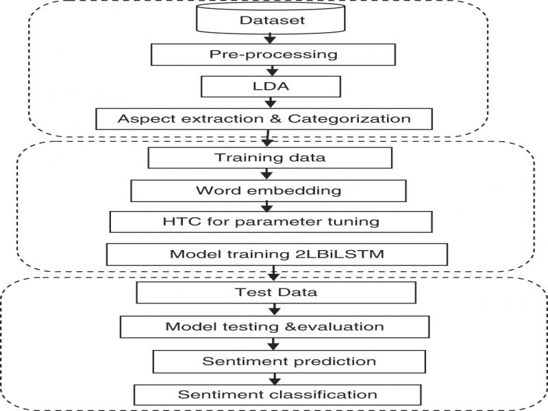
Figure 1:
The flow of the proposed algorithm.
Algorithm 1: Aspect Extraction
Input: Review dataset DS
Output: Aspect list with categories.
Input review corpus and pre-process it.
Tokenize pre-processed corpus into words.
Remove outliers from tokenized words.
Create a Bag of Words (BOW) representation.
Apply LDA on BOW to get topic-word probability distribution.
Apply POS rules on LDA output distribution to get the most probable aspects.
Categorization of aspects into various categories is done through domain knowledge and frequent cohesive terms.
Based on step 7, categories review sentences into the aspect category.
Algorithm 1 produces various categories of aspect sentences that are labeled as positive and negative. The aspect list generated using Algorithm-I expanded using frequent corpus terms and domain knowledge. The aspect expansion helps cover more reviews, and aspect categorization gives a better picture of various aspects. Now we pass these categories data into our RNN model for sentiment classification.
Bi-LSTM model’s hyperparameters are tuned using hill-climbing tuning (HCT) algorithm. HCT picks the best direction in the hyperparameters space to choose the next hyperparameter value at each iteration. The optimization loop ends if no neighbor enhances the accuracy of the model. Figure 2 shows the flow of algorithm 2.
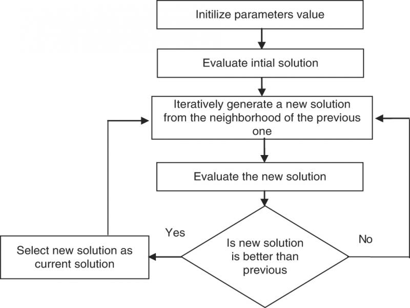
Figure 2:
Flow of the proposed HCT algorithm.
The formal description of the HCT algorithm is as follows:
Algorithm 2: HCT algorithm for hyper-parameter tuning
Input: Test data (x_test, y_test), No of iterations n
initialize a list for out_val: list()
generate solution with random prediction on x_test: sol = ran_pred(x_test)
evaluate initial value & put on score list: eval_pred(y_test, sol)
append out_val
for i= 1 to n do:
append out_val // appending output value in a list
if out_val = 1 // already present in the list
break
candi = mod_pred(sol) // generating new candidate
val = eval_pred(y_test, candi) // evaluate
if val>= out_val // checking for the better value
sol, out_val = candi, val
Return sol, out_val
Algorithm 2 gives the optimal configuration for hyperparameter, which offers improved accuracy of the model. Now we can proceed with the classification task using our Bi-LSTM model, which is explained in Algorithm 3.
Algorithm 3: Two-layer HCT Bi-LSTM Algorithm for sentiment classification.
Input: Dataset DS, DS divides into training and testing, i.e., DSTR and DSTS.
Output: Sentiment Classification of test data
for each category review, data DSTR do // Training of Bi-LSTM.
Import word vector set W from pre-trained word embedding //(Glove 100d)
Tuned model hyperparameters using HCT algorithm(Algorithm 2) // (learning rate, epoch etc.)
Initialize Bi-LSTM model hyperparameters with optimal values from step 3.
(classes, layers, epochs, document length, vocab)
for each review sentence, s ∈DSTRi do
get the word vectors s = [w1, w2, w3, w4…, wn‒1, wn] of all words in s from W
for Bi-LSTM forward pass, do
forward_pass for
i. f_state LSTM;
ii. b_state LSTM;
end of for
for Bi-LSTM Backward pass, do
backward_pass for
i. f_state LSTM;
ii. b_state LSTM;
end of for
representation sequence generated by the memory cell = [h1, h2, h3, h4…, hn‒1, hn];
vector h is generated by a max-pooling operation;
The output layer obtains the sentiment class of the input sentence
end of for
// Evaluating the model for test data
for each review sentence, s ∈DSSTSi do
get the word vectors s = [w1, w2, w3, w4…, wn‒1, wn] of all words in s from W
for Bi-LSTM forward pass, do
f_state LSTM;
b_state LSTM;
end of for
for Bi-LSTM Backward pass, do
f_state LSTM;
b_state LSTM;
end of for
Representation sequence generated by the memory cell = [h1, h2, h3, h4…, hn‒1, hn];
Vector h is generated by a max-pooling operation;
The output layer obtains the sentiment class of the input sentence
end of for
classified test data.
End:
Steps 7 to 9 represent the forward pass for Bi-LSTM. Except the input sequence is presented in opposite directions to the two hidden layers, it is equivalent to unidirectional LSTM, and the output layer is not changed until both hidden layers have interpreted the whole input sequence. Steps 10 to 12 represent the backward pass for Bi-LSTM. Except that all the output layer and terms are first determined, then fed back to the two hidden layers in opposite directions for all t, Backward passes for the output layer in any order, storing and terms at each stage. It is comparable to unidirectional LSTM.
Experimental setup and results
Environment and system configuration
The Gensim implementation of LDA on the Anaconda platform is used for Python. The tests on Core I5 CPU @ 2.5 GHz 2.49 GHz with 8 GB of RAM were performed on Windows 8 OS. For implementing Bi-LSTM Model in Python, Tensor-Flow with Keras is used. For performing pre-processing in Python sci-kit-learn library is used.
Datasets
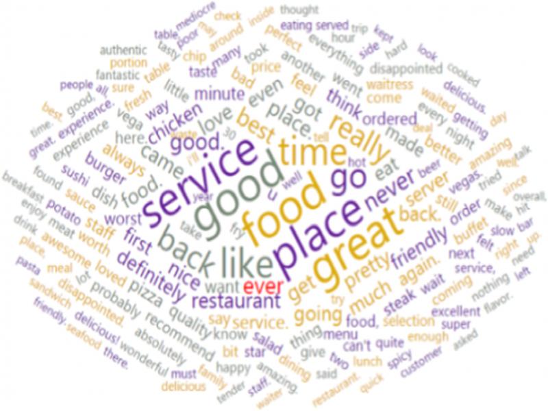
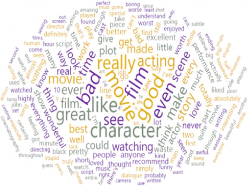
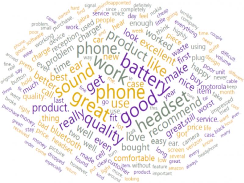
We have used three different datasets for the evaluation of our algorithm. Kaggle has provided a labeled Sentences Data Set, publicly available by the University of California for Sentiment Analysis (https://www.kaggle.com/rahulin05/sentiment-labelled-sentences-data-set). Table 1 gives the detail about the datasets.
Table 1.
Dataset statistics.
| Dataset domain | Total | +ve | ‒ve | |||
|---|---|---|---|---|---|---|
| Restaurant from Yelp | 1,000 | 500 | 500 | |||
| Mobile from Amazon | 1,000 | 500 | 500 | |||
| Movies from IMDB | 1,000 | 500 | 500 | |||
| Parameter | Value | |||||
|---|---|---|---|---|---|---|
| Vocabulary size | 10,000 | |||||
| Bi-LSTM | 2 layer | |||||
| Dense | 1 | |||||
| Activation | Sigmoid | |||||
| Optimizer | Adam function | |||||
| Loss Function | Binary cross-entropy | |||||
| Input Length | 100 | |||||
| Learning rate | 0.002 | |||||
| Epoch | 10 | |||||
| Model | Single-layer Bi-LSTM (Hameed and Garcia-Zapirain, 2020) | Two-layer Bi-LSTM | Two-layer HCT Bi-LSTM | |||
|---|---|---|---|---|---|---|
| Dataset | T | V | T | V | T | V |
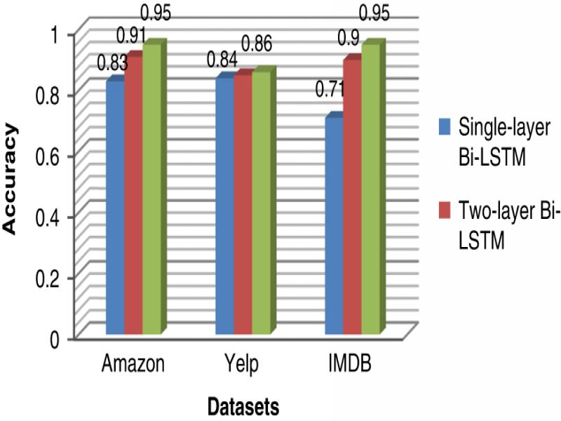
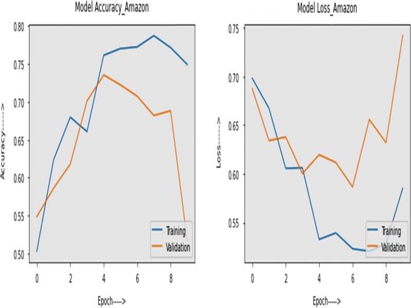
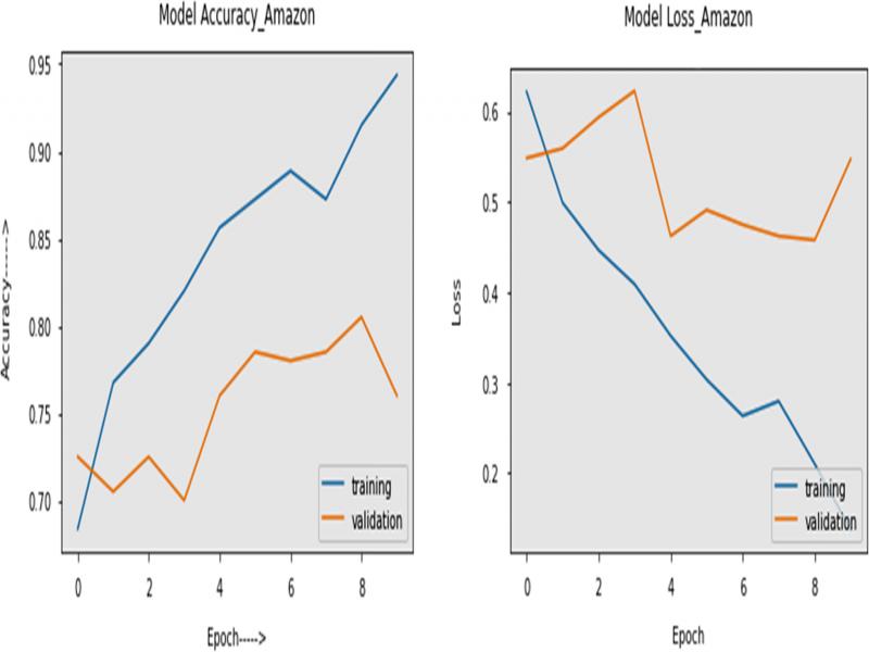
| Amazon | 0.83 | 0.51 | 0.91 | 0.70 | 0.95 | 0.76 |
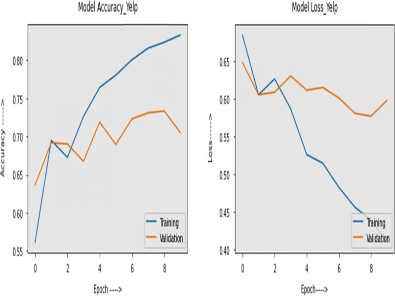
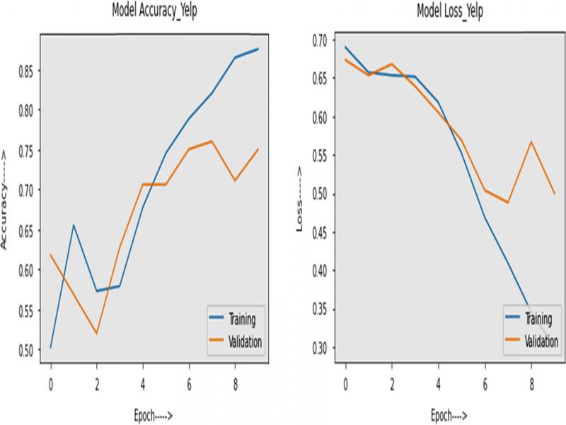
| Yelp | 0.84 | 0.70 | 0.85 | 0.72 | 0.86 | 0.75 |
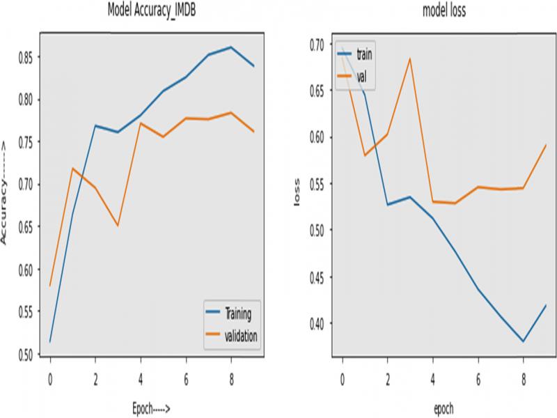
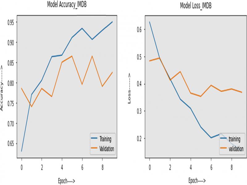
| IMDB | 0.71 | 0.81 | 0.90 | 0.81 | 0.95 | 0.82 |