
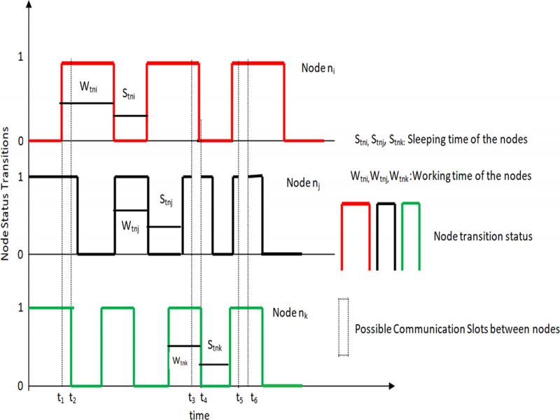
Figure 1:
Asynchronous work-sleep cycle approach for nodes in the network.
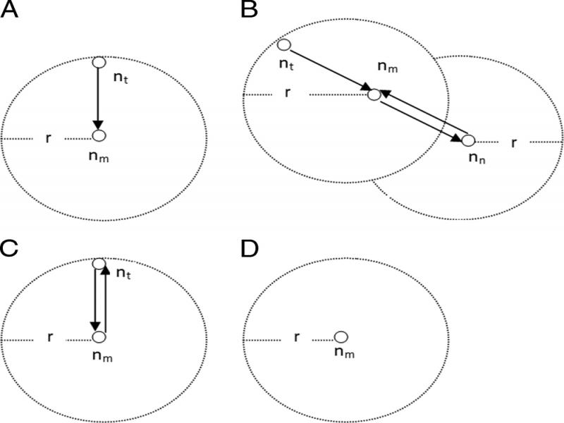
Figure 2:
Illustration of probe message transmission.
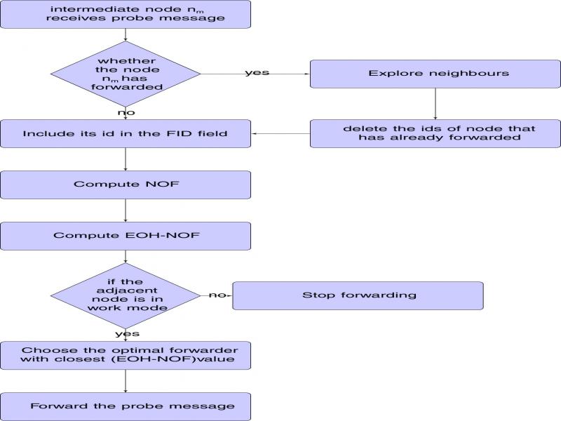
Figure 3:
Probe message transmission.
Table 2.
Fuzzy I/O variables and their linguistic terms.
| I/O variables | Linguistic variables |
|---|---|
| Residual energy of node (NRE) | Low, Medium, High |
| Queue size (QS) | Low, Medium, High |
| Status transition frequency (STF) | Low, Medium, High |
| Link quality (LQ) | Poor, Moderate, Good |
| Possibility of turning into subsequent node for hopping | Low, Weak, Medium, High, Very high |
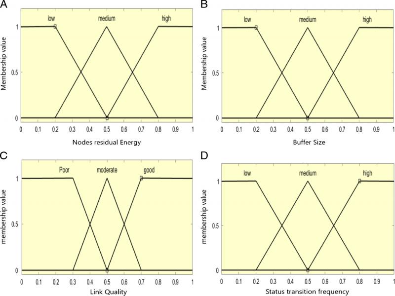
Figure 4:
Membership functions for input variables.
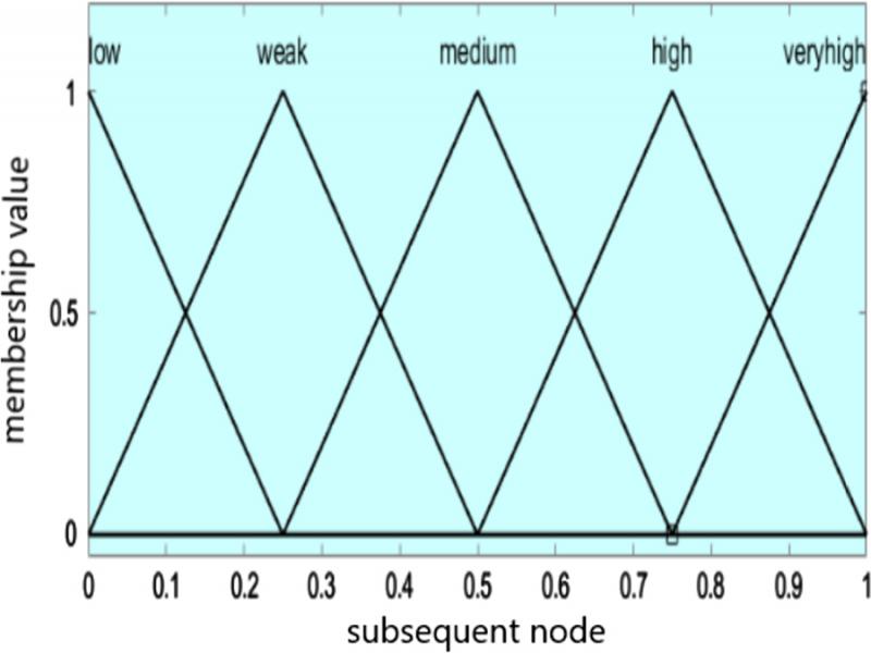
Figure 5:
Membership function for output variables.
Table 3.
Fuzzy decision rules.
| Residual energy | Queue size | STF | Link quality | Chance of becoming subsequent node |
|---|---|---|---|---|
| Low | Low | Low | Poor | Low |
| Low | Low | Low | Moderate | Low |
| Low | Low | Low | Good | Weak |
| Low | Low | Medium | Poor | Low |
| Low | Low | Medium | Moderate | Medium |
| Low | Low | Medium | Good | Medium |
| Low | Low | High | Poor | Weak |
| Low | Low | High | Moderate | Weak |
| Low | Low | High | Good | Medium |
| Low | Medium | Low | Poor | Low |
| Low | Medium | Low | Moderate | Low |
| Low | Medium | Low | Good | Low |
| Low | Medium | Medium | Poor | Low |
| Low | Medium | Medium | Moderate | Weak |
| Low | Medium | Medium | Good | Medium |
| Low | Medium | High | Poor | Low |
| Low | Medium | High | Moderate | Weak |
| Low | Medium | High | Good | Medium |
| Low | High | Low | Poor | Low |
| Low | High | Low | Moderate | Low |
| Low | High | Low | Good | Low |
| Low | High | Medium | Poor | Low |
| Low | High | Medium | Moderate | Weak |
| Low | High | Medium | Good | Medium |
| Low | High | High | Poor | Weak |
| Low | High | High | Moderate | Medium |
| Low | High | High | Good | High |
| Medium | Low | High | Poor | Low |
| Medium | Low | High | Moderate | Low |
| High | Low | Low | Poor | Low |
| High | Low | Low | Moderate | Low |
| High | Low | Low | Good | Weak |
| High | Low | Medium | Poor | Low |
| High | Low | Medium | Moderate | Weak |
| High | Low | Medium | Good | Medium |
| High | Low | High | Poor | Low |
| High | Low | High | Moderate | Weak |
| High | Low | High | Good | Medium |
| High | Medium | Low | Poor | Weak |
| High | Medium | Low | Moderate | Medium |
| High | Medium | Low | Good | High |
| High | Medium | Medium | Poor | Medium |
| High | Medium | Medium | Moderate | High |
| High | Medium | Medium | Good | Very High |
| High | Medium | High | Poor | Medium |
| High | Medium | High | Moderate | High |
| High | Medium | High | Good | Very High |
| High | High | Low | Poor | Weak |
| High | High | Low | Moderate | Medium |
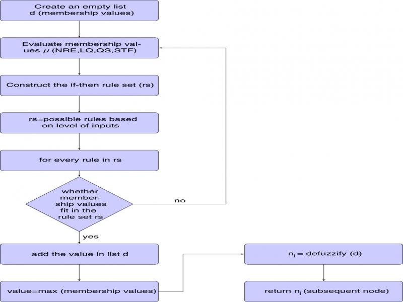
Figure 6:
Subsequent hop node selection.
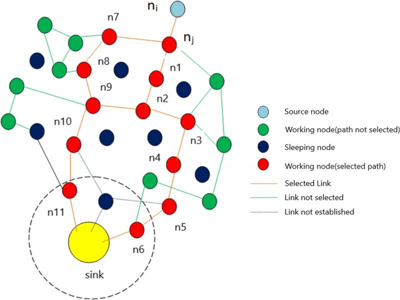
Figure 7:
Multi disjoint path selection for data communication on the spanning tree.
Table 4.
Simulation attributes.
| Parameters | Values |
|---|---|
| Size of the network | (500 × 500) m2 |
| No of mobile sink | 1 |
| No of nodes in the network | 500 |
| Mobility pattern | random |
| Time duration for data collection | 600 s |
| Communication range between sensor nodes | 20 m |
| Node’s initial energy | 2 J |
| Size of the buffer | 1,024 bits |
| Eelec | 50 nJ/bit |
| E | 0.0013 pJ/bit/m4 |
| Size of probe message | 120 bits |
| Size of data packet | 1,024 bits |
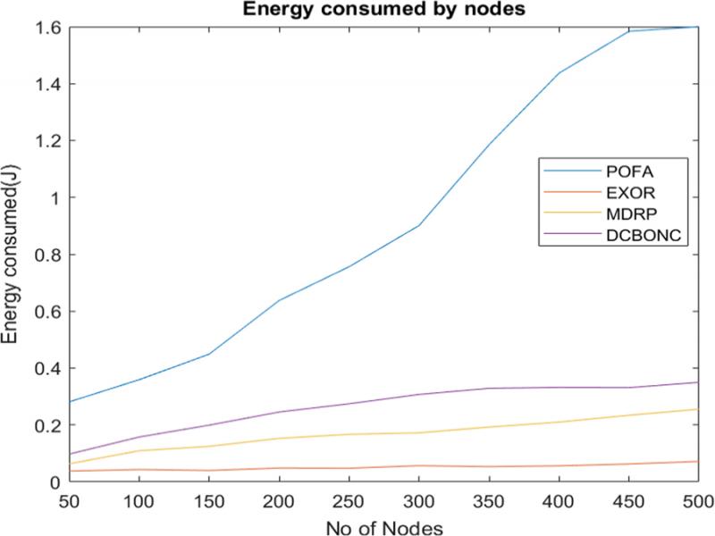
Figure 8:
Energy consumed by nodes in the network.
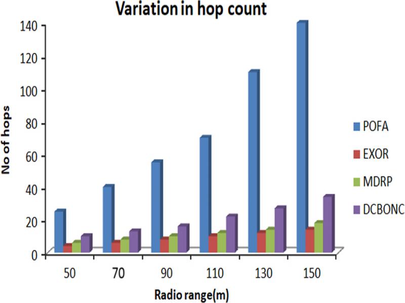
Figure 9:
Hop count variation with increase in radio range.
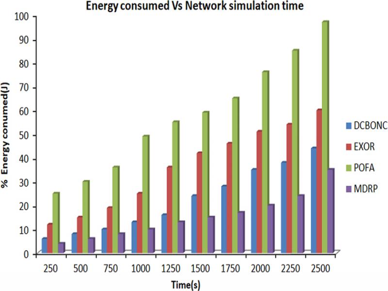
Figure 10:
Energy consumed vs network simulation time.
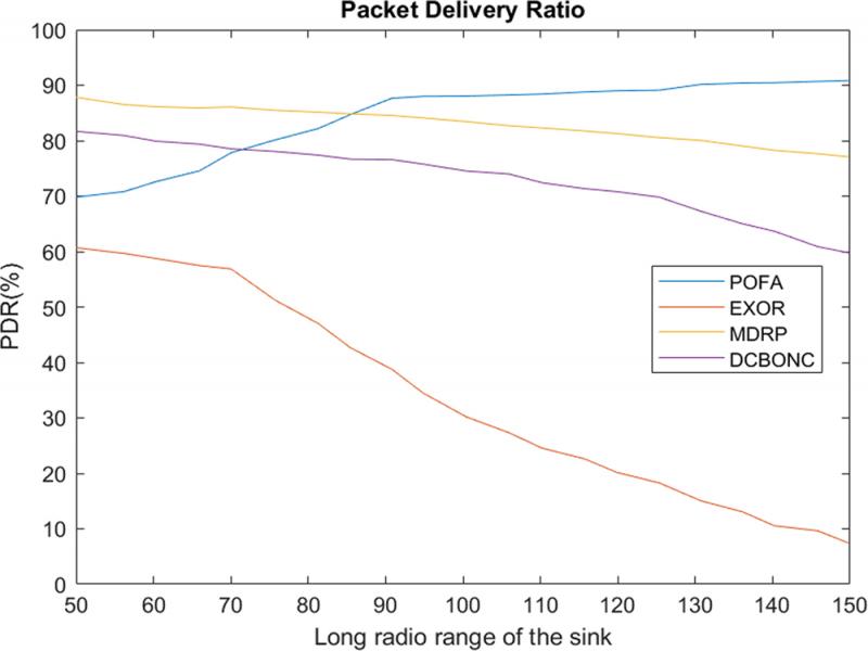
Figure 11:
Packet delivery ratio.
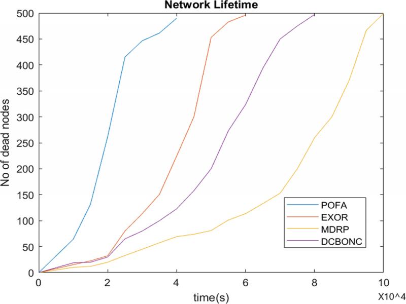
Figure 12:
Network lifetime.
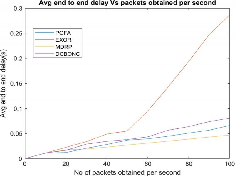
Figure 13:
Avg end to end delay.