The quadrotor unmanned aerial vehicle (UAV) is an autopilot aircraft vehicle that is driven without a human pilot onboard. Previously, the quadrotors manufactured were of big sizes, which were highly costly and expensive. Fortunately and due to recent progress in the technologies in the batteries, electronics kits, mechanics, the quadrotors now manufactured are of small sizes, with affordable prices. In terms of the mathematical modeling of the quadrotor systems, the Newton–Euler method is the most commonly applied for driving the quadrotor model (Lee et al., 2011; Naidoo et al., 2011; Rodić and Mester, 2011; Chovancová et al., 2014).
Numerous representations of the quadrotor dynamics modeling and control algorithm have been presented, and the desired pitch and roll angles are calculated by using the virtual control method (Alkamachi and Erçelebi, 2017; Lee and Kim, 2017; Eltayeb and Rahmat, 2019). The quadrotor system has nonlinear dynamics, underactuated, and unstable system; these issues must be counted while developing the control algorithms. Numerous control methods have been implemented for the quadrotor systems in the literature, for instance, the PID controller, which is extensively applied to the quadrotor systems (Min et al., 2009; Salih et al., 2010; Li and Li, 2011; Khatoon et al., 2014; Romero et al., 2016; Abdulwahhab and Abbas, 2017).
The quadrotor’s dynamic is linearized at the equilibrium points, then the controllability and observability verified of the obtained linear model (Ataka et al., 2013; Al-Younes et al. 2010). The dynamics of quadrotor is divided into three subsystems: attitude, altitude, and positions to design the backstepping and augmented backstepping controller (Madani and Benallegue, 2006; Behnamgol et al., 2016; Zhang et al., 2017). The direct feedback linearization and adaptive feedback linearization for quadrotor are designed (Lee et al., 2009; Mukherjee and Waslander, 2012). The attitude controller is designed based on quantitative feedback theory; then, a fuzzy logic controller is implemented to provide the position trajectory tracking for the quadrotor UAV (Mukherjee and Waslander, 2012; Figueroa-García et al., 2017; Mardan et al., 2017).
The sliding mode control (SMC) is classified among robust and simple control techniques for the types of nonlinear dynamics such as the quadrotor system and its robustness against the parameter uncertainties and external disturbances (Bartolini et al., 2003). The quadrotor systems operate in the harshness environment, which leads to real challenges such as the parameter uncertainties and external disturbance in the quadrotor dynamics (Abaunza et al., 2016). Many types of SMC controllers have been reported in the literature to deal with the prior mentioned challenges, such as given in Eltayeb et al. (2020), Patel et al. (2012), Runcharoon and Srichatrapimuk (2013). The disadvantage of the conventional SMC controller is the chattering problem, which can be reduced by using the augmented the SMC approach such as adaptive SMC, fuzzy SMC control, and intelligent SMC control (Lee and Utkin, 2007; Boiko, 2013; Sahamijoo et al., 2016; Baghaei et al., 2017).
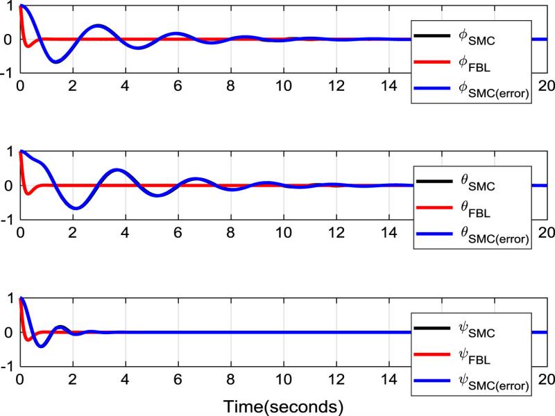
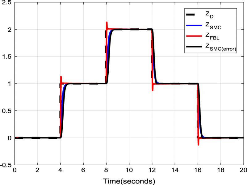
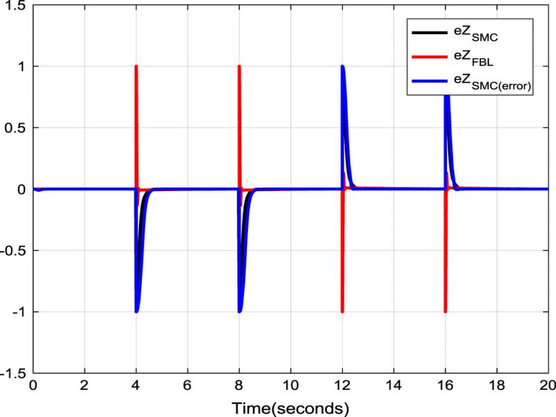
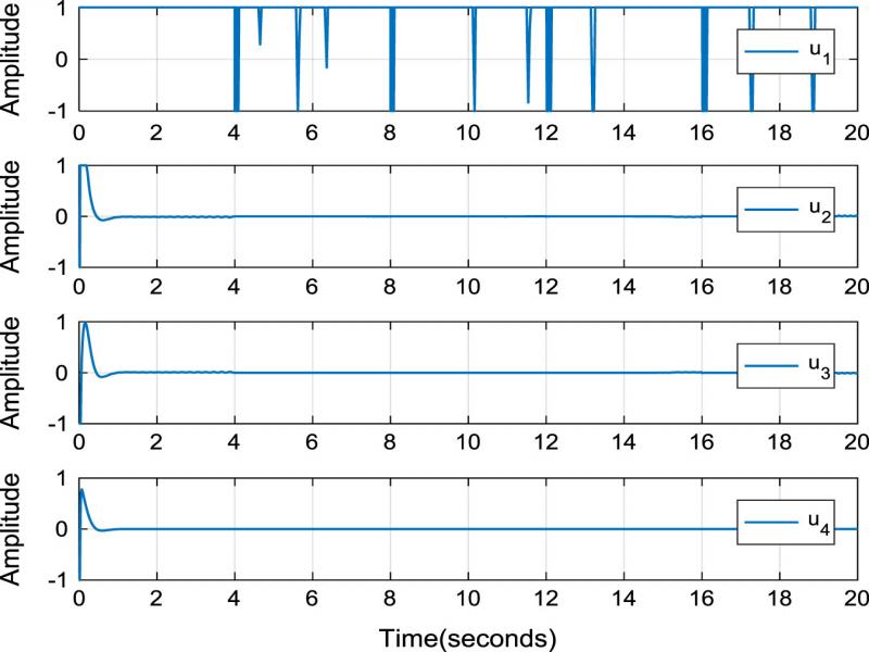
In this manuscript, a dynamic model of quadrotor UAV has been briefly presented. The feedback linearization method has been used to linearize the quadrotor’s attitude and altitude dynamic. The PID controller is applied to the linearized quadrotor model. For the robust performance against uncertainty in quadrotor’s mass, a proposed (SMC) controller has been designed to stabilize the quadrotor’s attitude and altitude and reduce the chattering impact as well. Finally, the proposed control technique has been validated by simulation using Matlab/Simulink environment.
The paper is organized as follows: the first section is the introduction, which presents some previous and related works. Second section presents the quadrotor UAV mathematical modeling briefly. The third section explains the design and implementation of the proposed control strategy for the quadrotor’s attitude and altitude, along with the chattering reduction technique, in addition to the traditional SMC and feedback linearization controller as the benchmark. The fourth section presents the simulation results to evaluate the proposed SMC controller performance, and fifth section concludes the work with some recommendations and future work.
Quadrotor modeling
Quadrotor UAV model description
The quadrotor UAV comprises of four rotors to produce the forces (F1, F2, F3, F4). The rotors are fixed in a cross structure and symmetric shape, as illustrated in Figure 1.
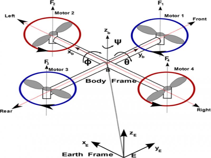
Figure 1:
Quadrotor UAV configuration.
The quadrotor motions are controlled by changing the speed of the rotors. The front and the rear of the quadrotor are represented by the rotors 1 and 3, and the left and the right are represented by the rotors 2 and 4, as depicted in Figure 1. By agreement, the rotors 1 and 3 turning in the clockwise direction, whereas rotors (2 and 4) turning in to the counterclockwise direction.
The quadrotor moves in a vertical direction by increasing or decreasing the angular velocities of all rotors with equal speed, which generates a total lift force (thrust) against the gravitational force. Consequently, the quadrotor takes-off or lands, as illustrated in Figure 2a and b, respectively.
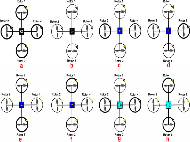
Figure 2:
Motions of the quadrotor UAV system.
The right direction movement of the quadrotor is achieved by increasing the rotational speed of the rotor (2) and decreasing the rotational speed of the rotor (4); subsequently, the quadrotor moves in the right direction as depicted in Figure 2c. Likewise, the left direction movement is achieved by increasing the rotational speed of the rotor (4) and decreasing the rotational speed of the rotor (2); as a result, the quadrotor moves to the left direction as shown in Figure 2d.
The forward movement of the quadrotor is achieved by increasing the rotational speed of the rotor (3) and decreasing the rotational speed of the rotor (1); subsequently, the quadrotor moves to the forward direction as illustrated in Figure 2e. Similarly, the backward movement of the quadrotor is achieved by increasing the rotational speed of the rotor (1) and decreasing the rotational speed of the rotor (3); as a result, the quadrotor moves to the backward direction as shown in Figure 2f. The anti-clockwise and clockwise movements of the quadrotor are controlled by changing the yaw angle (ψ) as shown in Figure 2g and h, respectively.
Quadrotor UAV kinematic model
The quadrotor kinematics are represented into two frames. The earth fixed, or the reference frame (E-frame), is denoted by E = (xe, ye, ze) and the body-fixed (B-frame) is represented by B = (xb, yb, zb) as shown in Figure 1.
Consider that q = (x, y, z, ϕ, θ, ψ) ∈ R6 denotes the generalized coordinates, with (x, y, z) representing the position the quadrotor and ϕ, θ, ψ representing the quadrotor’s orientation. Accordingly, the quadrotor mathematical model can be divided into two subsystems: the position and the attitude subsystems, and the associated coordinates are given as follows:
(1)where:(2)and:Therefore, the quadrotor kinematics are obtained as follows:
where V denotes the linear velocity in the B-frame, whereas ξ represents the linear velocity in the E-frame with respect to B-frame, and R is the rotation matrix:The quadrotor rotational motions are obtained as the following:
where ω denotes the angular velocity for the B-frame, whereas denotes the angular velocity for the E-frame with respect to the B-frame, and T is the transfer matrix (Olfati-Saber, 2001):Quadrotor dynamic model
The quadrotor dynamics equations in six degrees of freedom (6 DOFs) are given as follows:
where u1, u2, u3, u4 represent the control inputs, which calculated as follows:while Ωd denotes the disturbance, and mathematically expressed as follows:The control inputs in (9) can be re-written in the matrix as:
Control design
Feedback linearization
The feedback linearization technique is used to transfer the nonlinear systems to the equivalent linear systems, as illustrated in Figure 3 (Eltayeb et al., 2019, 2020).
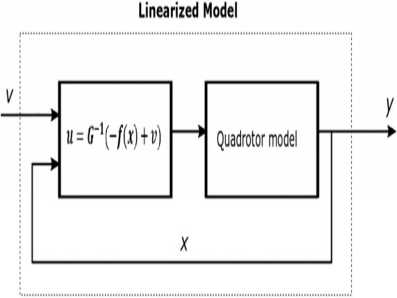
Figure 3:
The block diagram of the feedback linearization (FBL).
Now, consider the general nonlinear system expressed as:
(12)where f(x) is the nonlinear function; x is the system’s state vector; and u is the control input.The control input u in (12) can be chosen as:
By substituting (13) into (12) yields to the following linear system:
Now, by following the same prior steps from (12) to (14), the control inputs u1, u2, u3 and u4 in (8) of the quadrotor attitude and altitude can be chosen as in (15):
where:Thus, from (8) and (15), the quadrotor’s attitude and altitude systems are obtained in the linearized version as follows:
The obtained linear system in (16) can be represented in the state space as follows:
(17)where the output of the linear system is:(18)and:and the system’s states are:Now, the objective is to design the PID control strategy to stabilize and control the quadrotor linear system (17). The errors dynamics are defined as follows:
where eϕ, eθ, eψ, and ez are the errors signals for roll, pitch, yaw, and the altitude, respectively. ϕd, θd, ψd, and Zd are the desired signals for roll, pitch, yaw, and the altitude, respectively.Thus, the PID control is designed and implemented for each as follows:
where i = 1, 2, 3, 4, and Kp⩾0, KI⩾0, and KD⩾0 represent the PID controller parameters; vi is the PID generated control signal.The sliding mode control (SMC)
The SMC control technique uses to attract the state variables of the system towards the equilibrium sliding surface and stay on it. The sliding surface can be designed as follows (Vaidyanathan and Lien, 2017):
where s(t) ∈ Rn is the equilibrium surface; e(t) is the error between the desired and actual position or orientation; and k is a positive constant; and n ∈ N is the system’s order. SMC control can be designed as follows.First, select a Lyapunov function (candidate function) which maps the system’s state variables as follows:
Second, the derivative of the selected function (22) must be negative:
(23)yields to:The sliding mode control law consists of two terms: continuous part and the discontinuous part, which is given as follows (Herrera et al., 2015):
From (24), sliding mode condition given as follows:
(26)where k1>0 and k2>0 are the SMC design parameters.Chattering reduction
Chattering is an unwanted phenomenon with a finite-frequency, and finite-amplitude oscillations happened near to the sliding surface (Al-Younes et al., 2010). The chattering is caused by the switching function; therefore, in this work, the switching function (sing(s)) in the SMC control laws has been replaced by an approximated error function, as shown in Figure 4. The error function is obtained by integrating the normalized Gaussian distribution as follows (Eltayeb et al., 2020):
(27)and it has the following properties: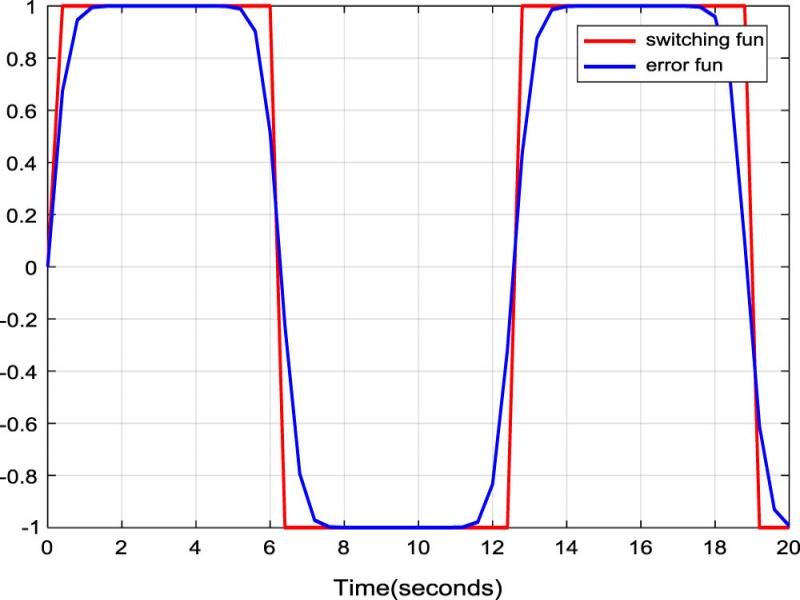
Figure 4:
Simulated switching (sign) function against error (erf) function.
SMC control design for the quadrotor
The SMC controller is designed to stabilize the quadrotor’s attitude and altitude.
The first step is to design the error dynamics as in (19).
The second step is to choose the sliding surfaces as the following:
(28)where , and represent the surfaces of the roll, pitch yaw, and altitude dynamics, respectively. , and are the SMC controller parameters.The third step recalls the sliding mode condition as in (26) and applies it to (28) to compute the SMC control laws.
The steps, as mentioned above, will be implemented to calculate the SMC control law (u1) for the roll angle as follows:
(29)where and are the SMC control parameters of the controlled variable .By substituting (8) into (29), the SMC control law for the roll angle () is driven as in (30):
Similarly, the SMC control laws for pitch, yaw, and altitude (), (), and (), respectively, are obtained as follows:
(31)(32)Therefore, to reduce the chattering effects, which leads to critical problems such as vibration in the mechanical parts of the quadrotor and heat in the onboard electronics kits (Li et al., 2014). The switching function (sign(s)) has been replaced by the error function erf(s) in the proposed SMC control laws as follows:
(34)(35)(36)Simulation model
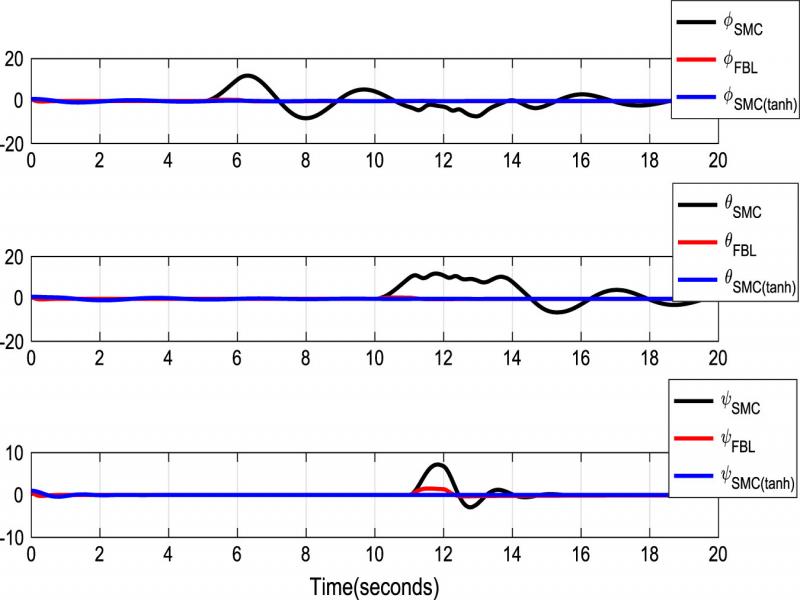
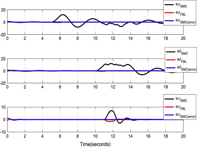
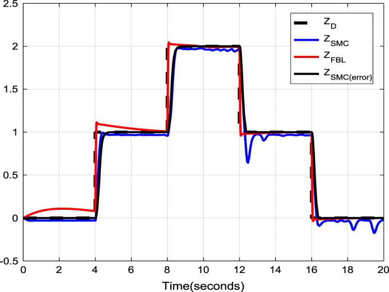
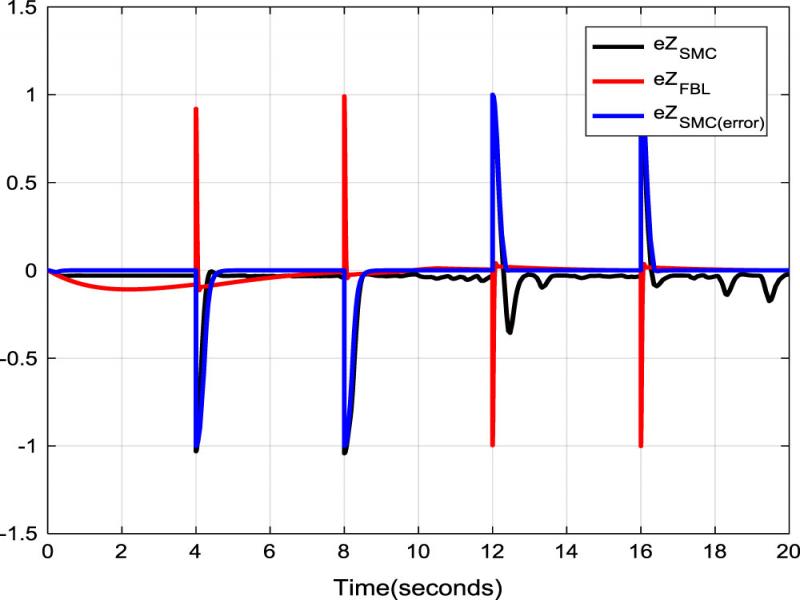
The quadrotor UAV model in (8) has been simulated using Matlab/Simulink platform, and the quadrotor’s parameter values are taken from Bouabdallah (2007) as listed in Table 1. The PID and SMC controller’s parameters are listed in Tables 2 and 3, respectively.
Table 1.
Parameters of the quadrotor model.
| Description | Symbols | Values | Units | |
|---|---|---|---|---|
| The quadrotor’s mass | m | 65 × 10−2 | kg | |
| x-axis inertia | Ix | 7.5 × 10⁻³ | kgm2 | |
| y-axis inertia | Iy | 7.5 × 10⁻³ | kgm2 | |
| z-axis inertia | Iz | 1.3 × 10⁻² | kgm2 | |
| Thrust coefficient | b | 3.13 × 10⁻⁵ | Ns2 | |
| Drag coefficient | d | 7.5 × 10⁻⁷ | Nms2 | |
| Inertia of the rotor | Jr | 6 × 10⁻⁵ | kgm2 | |
| Length of the arm | l | 23 × 10−2 | m |
| Parameter | z | |||
|---|---|---|---|---|
| P | 30 | 30 | 30 | 60 |
| I | 8 | 8 | 8 | 20 |
| D | 8 | 8 | 8 | 80 |
| Parameter | 𝝓 | 𝜽 | 𝝍 | z |
|---|---|---|---|---|
| k | 100 | 100 | 100 | 0.001 |
| k1 | 10 | 10 | 10 | 10 |
| k2 | 10 | 10 | 10 | 10 |