ECG is the most significant physiological signals, which can be extracted from heart activity, it is represented the activity of the heart, this activity is represented as electrical graph, this graph can be provided most important information, which is used to diagnosis the heart (Saxena et al., 2002; Merino et al., 2015). The ECG signal can be summarized by consecutive waves and most significant of them are P-wave, QRS wave and T-wave, which represented the characteristics of the signal. P-wave represent a trial depolarization and the distance between beginning of P-wave and the beginning of QRS is called PR interval, which serves as baseline for curve of ECG, PR amplitude is a measure for deflection/wave. QRS complex reflect depolarization of ventricles and its duration time is start from P-wave to the end of QRS, while the T-wave represented rapid repolarization of cells of contractile, the normal T-wave is asymmetric, the time from starting of QRS to the end of T- wave is called QT interval, the detail description of the ECG is shown in (Fig. 1) (Haddadi et al., 2014).
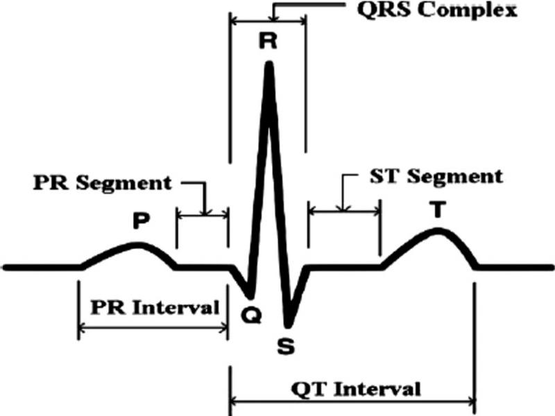
Figure 1:
ECG signal structure.
The QRS represented significant part of the ECG signal, so it was named as the reference waveform for ECG signals, because it can be used to evaluate the characteristics of the whole signal, so accurate detection was affected the efficiency of ECG analyzing algorithm, also the interval between R–R time can be calculated and rated of heart is determined (Chan et al., 2005).
The basic part of QRS complex is R peak, so it is the basic part of the signal for detecting the QRS complex, so it is very necessary to detect the location of R-peak from the signal accurately. After determined the location of R peaks, The other components of the signal such as P and T waves can be computed depending on the R peak according to their location with respect to QRS complex (Laguna, 1994). Because ECG signals are exposed by different types of noises and artifacts (Gargasas et al., 2004; Wu et al., 2009), different algorithms and methods are used to de-noising and reprocessing it, this can increase the accuracy of ECG analysis.
Discrete wavelet transform (DWT) is consider very useful method in preprocessing of medical signal, it is always uses for low frequency signal analysis. DWT can separate the high frequency from the low component, and this facilitates are the handling with low and high frequencies separately, so each part can be treated separately. In this paper, we have proposed a new technique to detect QRS by using DWT (Haddad et al., 2017), in which the DWT can be used to de-noise the original ECG signal by using threshold method that is applied to details coefficients of the wavelet transform, also DWT is used to determine the statistics of the approximation coefficient (low frequency components) that can be used to calculate the threshold that is used in detection method. The main contributions of our work is that, We used statistical information of the signal to find the threshold, depending on wavelet transform in which, the great information is founded in approximation sub-band, while the details components have less influence on the curve of the ECG signal, so its statistical is less significant in threshold computation.
Literature survey
There are many researches and studies are performed for detection of QRS complex peaks, some of which can be listed as following.
In 2013, Xiaoran Ning and Ivan W. Selesnick proposed method for detection QRS complex based on sparse derivatives. The proposed system is used the filter (8-20 Hz) to pass band in order to discard high-frequency noise and baseline wander noise. Then this signal is converted into segment, Hilbert transform is used as first-order derivative, then variable threshold was calculated according to the mean square error value. Then QRS is detected as the maximum value in the specified samples (Ning and Selesnick, 2013).
In 2017, Jeong-Seon Park et al. proposed algorithm to detect QRS complex based on DWT, which is applied to eliminate the noise and generate Shannon energy envelope after applying first-order differentiation, which is accomplished by using first-order filter (high pass filter) then amplitude normalization was used. They extract peak energy envelope from the created Shannon energy envelope, the final peaks are extracted from these peak energy envelope, also their system is used to determine R features based on R–R time, also they used different types of filters to smooth the signal through different stage of the algorithm (Park et al., 2017).
In 2017, Runnan He1 et al. proposed QRS detection algorithm in a real-time. In this technique, baseline noise is removed from the signal by band-pass filter. Then, recognition method is constructed from combining (KNN) and (PSO) methods, which are used to select the parameters, this optimization can increase the accuracy for QRS complex detection. Also, in this work, first-order differentiation with five point filter was used to increase the features of the QRS complex and enhance the signal (Runnan et al., 2017).
In 2018, Suleyman and Zahide Elif proposed method for detection of QRS by using digital filtering and DWT, at first, they used SGF method (Savitzky–Golay filtering), which is applied on the signals obtained from the database, this method suppress the high frequency components. After that, BPF is used in order to isolate the P-wave and T waves and make QRS distinct, then DWT method was applied to increase the prominent of QRS. The recognition of zones of QRS is satisfied by modified threshold. Also they used (HPF) in their system to remove the signal baseline noise (Billgan and Akin, 2018).
In 2019, Alka Barhatte et al. proposed used curvelet transform with an adaptive threshold to detect the interest region and guess the R-peak boundaries. Then, they determine the exact location of R-peak depending on estimated boundaries. They used curvelet energy, which is applied to the ECG signal, then threshold is used to determine the region of interest, which contain R peaks for the ROI, then false peaks are removed to increase the accuracy, also there are two threshold in the work, which are lower and upper threshold, these threshold are updated according to the number of peaks (Barhattei et al., 2018).
Methodology
In this paper, we have proposed a new system depending on wavelet transform and variable threshold for ECG peak detection, the wavelet transform is used for signal enhancement and to compute the statistical of the approximation, which represented the low frequency components, this statistical will be used in the adaptive proposed threshold for peak calculation. The proposed system is described in Figure 2.
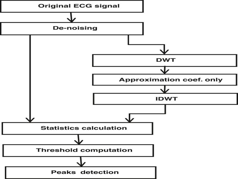
Figure 2:
Flowchart of the proposed method.
In statistics calculation, de-noised signal along with modified de-noised signal (which is obtained after applying DWT, discarding detail coefficients of wavelet transform and applying IDWT) are used to compute thresholds, which are used to detect peaks of the ECG signal.
ECG signal de-noising
We used wavelet transform to separate the information of signal into low frequency components (approximation sub-band) and high frequency component (less information or details), then, the proposed threshold is applied to the detail coefficients to reduce the noise, while the approximation coefficients will remain unchanged. The proposed threshold method is summarized in Algorithm I.
 where j wavelet level (always two or three for best De-noising), detail is wavelet transform coefficients (high frequency component), 0.6745 constant (Galya and Krassimir, 2013).
Discrete wavelet transform (DWT)
The DWT is applied to the original signal to separate the approximation coefficients, which is used to reconstruct the signal, while the details component of the signal will be replaced by zero values to eliminate the value that can not be used to determine threshold, as shown in (Fig. 3).
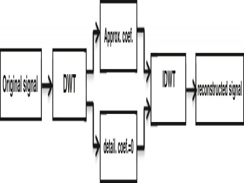
Figure 3:
Flowchart of signal reconstruction with approximation coefficients only.
Proposed algorithm for QRS detection:
The proposed threshold is based on the statistical computation of original signal along with the signal that was retrieved using the approximation coefficients and delete the detail coefficients after applying wavelet transform, the proposed algorithm can be summarized as following:
Step 1. Determine the ECG signal statistics mean, maximum and standard deviation and named as, meanori, maxori and stdori, respectively.
Step 2. Apply DWT to the signal and get the approximation coefficients.
Step 3. Reconstruct the signal by using the approximation coefficient only and substitute the details coefficient with zero value (delete details coefficients), then determine the statistical values as, meanapp, maxapp and stdapp.
Step 4. Calculate the average of the above statistical parameters as following:
where, maxori, meanori and stdori are maximum, mean and standard deviation of original signal respectively, while, maxapp, meanapp and stdapp are maximum, mean and standard deviation of reconstructed signal after wavelet transform, respectively.Step 5. Compute the lower and upper threshold as in the following equations:
We used 0.05 constant to ensure low value for ThL, while 0.7 is used to ensure high value for ThU, also the weights for the statistics are given according to their significant, max represent the basic parameters to determine the peak, it is multiplied by 0.7, less important is mean, which is multiplied by 0.5, while the lowest significant is standard deviation, which is multiplied by 0.1. (0.05 and 0.07 are considered based on experiments).
Step 6. Determine the number of peaks with lower and upper threshold as N1 peak and N2 peak, respectively, while N1 peak and N2 peak are not equal, update thresholds by:
where Δ = ThU − ThL and α is constant, we use α = 0.2.Step 7. Correct the detected peaks by, first determine the R–R intervals and calculate average R–R interval, if there is no peak after (1.5 average R–R) reduce lower threshold, if there is peak after less than (0.75 average R–R) increase threshold and repeat steps (5 and 6).
Step 8. Compute R–R time for successive peaks by determine the number of samples between them, then compute hear rate (HR) as following:
Metric evaluation
To determine the efficiency of our system, four metrics were used, which are applied to test the system, these metric can be explained as following.
Sensitivity (Sen%)
This metric represent the ratio between the detected peaks to all peaks:
Positive prediction (+p%)
This metric represent the ratio of true prediction to all prediction peaks:
Detection error rate (DER%)
This ratio represent the total number of detected peaks incorrectly to detected peaks correctly:
Accuracy
Represent the ratio of true detected peaks (TP) to the total numbers of positive true and total positive:
where TP represented true detected peak, FN means negative false peaks and FP means peaks that false positive detected. The values of FP and FN are determined by comparing the detected peaks with actual peaks in data set, if there is actual peak and not detected then (FN = FN + 1, there is peak not detected, FN initially zero), if there is no actual peak and detected peak then (FP = FP + 1, there is false detected peak, FP initially zero).Results and discussion
The proposed algorithm is performed peak detection and its performance is evaluated by using two types of databases, which are long-Term ST database (LTSTDB) and European ST-T database (EDB), these database are sampled with 250 sample per second. The algorithm is implemented by using mat lab with cori7 processor. Figure 4 shows the de-noising results of two ECG signals after applying de-noising method, which is used DWT with level three and db4 filter with the adaptive threshold method, that is applied to detail coefficients of wavelet transform.
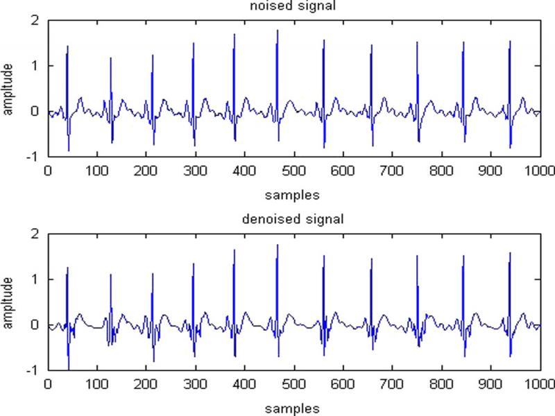
Figure 4:
De-noising of ECG signal.
The differences between reconstructed and original signal are by using approximation coefficients only is shown in Figure 5, it is clear that the approximation coefficient, which represented the most important part of the signal is represent the general shape of the signal without detail, which may give useful information to extract the peak of the signal.
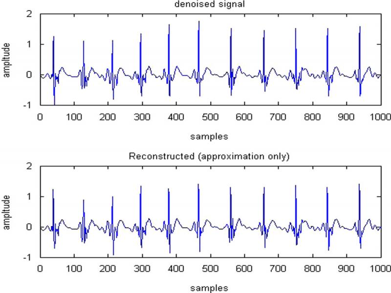
Figure 5:
The signal and its reconstruction using approximation coefficient only.
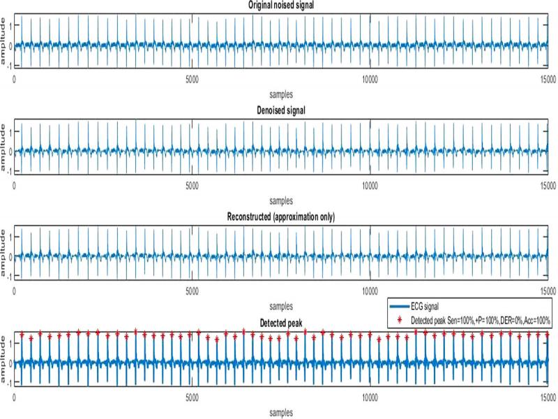
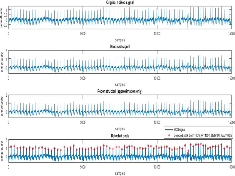
The proposed method is evaluated based on (LTSTDB) and (EDB) database for ECG signal, in which, we calculate TP, which represent true peak detection, FN means there is Peak founded but is not detected while FP, which means that the system is detect false peak. Based on these parameters, four metrics were calculated, which are sensitivity (Sen%), positive prediction (+P%), error detection rate (DER%) and accuracy (Acc%). Figure 6 shows the different stages of the proposed system results.
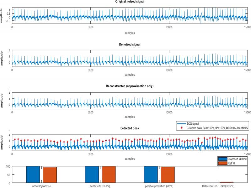
Figure 6:
Results of different stages of the proposed system.
As shown in Figure 6, all the peaks are detected correctly, in other word, all actual peaks are detected, no peak is detected incorrectly (FP = 0), also there is no actual peak not detected (FN = 0), according to these values, the proposed method achieved accuracy (100%), sensitivity (100%) and positive prediction (100%) with zero rate in (DER), which better than results of Park et al. (2017), which gives (93.97, 98.73 and 95.12%) for accuracy, sensitivity and positive prediction, also the DER is 6.4% in Park et al. (2017).
Results of LTSTDB dataset
The performance of the system is first tested by using LTSTDB database for 10 records with 1 min, which is shown in Table 1, there is very good improvement in sensitivity (Sen = 99.87%), positive prediction (+P = 99.628%) and accuracy (Acc = 98.89%), with very low value of error rate, which is (1.19), from Table 1, it is clear that all records in Sen, +P and accuracy are detected perfectly (100%) with zero value at DER, except record S20111m, which give lowest value in all metrics (95.23%), (98.76%) and (94.12%) for Sen, +P and Acc respectively, with 6.25 in DER rate.
Table 1.
R peak detection for (10) record with (1 min) for (LTSTDB) database.
| Record | Method | Actual peak | Detected peak | FP | FN | Sen(%) | +P(%) | DER(%) | Acc(%) |
|---|---|---|---|---|---|---|---|---|---|
| S20011m | Park et al. (2017) | 70 | 69 | 1 | 1 | 98.57 | 98.57 | 2.9 | 97.18 |
| Proposed | 70 | 70 | 0 | 0 | 100 | 100 | 0 | 100 | |
| S20021m | Park et al. (2017) | 72 | 71 | 1 | 1 | 98.61 | 98.61 | 2.8 | 97.26 |
| Proposed | 72 | 72 | 0 | 0 | 100 | 100 | 0 | 100 | |
| S20031m | Park et al. (2017) | 76 | 75 | 2 | 1 | 98.68 | 97.40 | 0.04 | 96.5 |
| Proposed | 76 | 76 | 0 | 0 | 100 | 100 | 0 | 100 | |
| S20061m | Park et al. (2017) | 92 | 92 | 2 | 0 | 100 | 97.87 | 3.2 | 97.87 |
| Proposed | 92 | 92 | 0 | 0 | 100 | 100 | 0 | 100 | |
| S20081m | Park et al. (2017) | 79 | 78 | 4 | 1 | 98.73 | 95.12 | 6.4 | 93.97 |
| Proposed | 79 | 79 | 0 | 0 | 100 | 100 | 0 | 100 | |
| S20091m | Park et al. (2017) | 106 | 105 | 0 | 1 | 99.06 | 100 | 0.95 | 99.05 |
| Proposed | 106 | 106 | 0 | 0 | 100 | 100 | 0 | 100 | |
| S20111m | Park et al. (2017) | 84 | 84 | 5 | 0 | 100 | 94.38 | 5.9 | 94.38 |
| Proposed | 84 | 80 | 1 | 4 | 95.23 | 98.76 | 6.25 | 94.12 | |
| S20121m | Park et al. (2017) | 60 | 60 | 3 | 0 | 100 | 95.24 | 5 | 95.63 |
| Proposed | 60 | 60 | 0 | 0 | 100 | 100 | 0 | 100 | |
| S20131m | Park et al. (2017) | 78 | 77 | 2 | 1 | 98.72 | 97.47 | 3.9 | 96.25 |
| Proposed | 78 | 78 | 0 | 0 | 100 | 100 | 0 | 100 | |
| S20571m | Park et al. (2017) | 91 | 90 | 3 | 1 | 98.90 | 96.77 | 4.4 | 95.74 |
| Proposed | 91 | 89 | 2 | 2 | 97.8 | 97.8 | 4.5 | 95.7 | |
| Total | Park et al. (2017) | 808 | 801 | 23 | 7 | 99.13 | 97.14 | 3.74 | 96.389 |
| Proposed | 808 | 804 | 3 | 6 | 99.87 | 99.628 | 1.19 | 98.89 |
| Beat no. number peak | R–R time | HR | Beat no. | R–R time | HR | ||||
|---|---|---|---|---|---|---|---|---|---|
| 1 | 0.9960 | 60 | 17 | 1.0200 | 59 | ||||
| 2 | 1.0240 | 59 | 18 | 0.9920 | 60 | ||||
| 3 | 1.0240 | 59 | 19 | 1.0160 | 60 | ||||
| 4 | 0.9920 | 60 | 20 | 1.0040 | 59 | ||||
| 5 | 1.0240 | 59 | 21 | 0.9840 | 60 | ||||
| 6 | 1.0000 | 60 | 22 | 1.0120 | 61 | ||||
| 7 | 1.0120 | 59 | 23 | 0.9800 | 59 | ||||
| 8 | 1.0240 | 59 | 24 | 1.0040 | 61 | ||||
| 9 | 1.0040 | 60 | 25 | 1.0000 | 60 | ||||
| 10 | 1.0080 | 60 | 26 | 0.9520 | 63 | ||||
| 11 | 1.0120 | 59 | 27 | 1.0120 | 59 | ||||
| 12 | 1.0160 | 59 | 28 | 0.9600 | 63 | ||||
| 13 | 1.0000 | 60 | 29 | 0.9880 | 61 | ||||
| 14 | 1.0200 | 59 | 30 | 0.9840 | 61 | ||||
| 15 | 1.0080 | 60 | 31 | 0.9840 | 61 | ||||
| 16 | 1.0120 | 59 | 32 | 0.9680 | 62 |
| Recored | Method | Actual peak | Detected peak | FP | FN | Sen(%) | +P(%) | DER(%) | Acc(%) |
|---|---|---|---|---|---|---|---|---|---|
| e0103m | Park et al. (2017) | 60 | 60 | 2 | 0 | 100 | 96.77 | 3.33 | 96.77 |
| Proposed | 60 | 60 | 0 | 0 | 100 | 100 | 0 | 100 | |
| e0104m | Park et al. (2017) | 72 | 70 | 1 | 2 | 97.22 | 98.59 | 4.16 | 95.89 |
| Proposed | 72 | 72 | 0 | 0 | 100 | 100 | 0 | 100 | |
| e0105m | Park et al. (2017) | 54 | 54 | 2 | 0 | 100 | 96.43 | 3.84 | 96.29 |
| Proposed | 54 | 54 | 0 | 0 | 100 | 100 | 0 | 100 | |
| e0106m | Park et al. (2017) | 57 | 55 | 1 | 2 | 96.49 | 98.21 | 5.45 | 94.82 |
| Proposed | 57 | 57 | 0 | 0 | 100 | 100 | 0 | 100 | |
| e0107m | Park et al. (2017) | 52 | 49 | 2 | 3 | 94.23 | 96.08 | 10.2 | 92.45 |
| Proposed | 52 | 52 | 0 | 0 | 100 | 100 | 0 | 100 | |
| e0108m | Park et al. (2017) | 54 | 54 | 3 | 0 | 100 | 94.74 | 5.55 | 94.73 |
| Proposed | 54 | 52 | 2 | 2 | 96.29 | 96.29 | 7.69 | 92.85 | |
| e0121m | Park et al. (2017) | 75 | 74 | 3 | 1 | 98.67 | 96.10 | 4.05 | 94.87 |
| Proposed | 75 | 75 | 0 | 0 | 100 | 100 | 0 | 100 | |
| e0166m | Park et al. (2017) | 51 | 50 | 0 | 1 | 98.04 | 100 | 2 | 98.04 |
| Proposed | 51 | 51 | 0 | 0 | 100 | 100 | 0 | 100 | |
| e0202m | Park et al. (2017) | 85 | 84 | 2 | 1 | 98.82 | 97.67 | 3.57 | 96.55 |
| Proposed | 85 | 85 | 0 | 0 | 100 | 100 | 0 | 100 | |
| e0818m | Park et al. (2017) | 69 | 69 | 2 | 1 | 98.55 | 97.14 | 4.16 | 95.83 |
| Proposed | 69 | 69 | 0 | 0 | 100 | 100 | 0 | 100 | |
| Total | Park et al. (2017) | 629 | 618 | 18 | 11 | 98.55 | 97.14 | 4.69 | 95.51 |
| Proposed | 629 | 627 | 2 | 2 | 99.682 | 99.682 | 0.318 | 99.366 |
| Beat no. number peak | R–R time | HR | Beat no. | R–R time | HR |
|---|---|---|---|---|---|
| 1 | 1.1440 | 52 | 17 | 1.0320 | 58 |
| 2 | 0.8720 | 69 | 18 | 1.0160 | 59 |
| 3 | 1.1400 | 53 | 19 | 1.0800 | 56 |
| 4 | 1.1000 | 55 | 20 | 1.1480 | 52 |
| 5 | 1.0800 | 56 | 21 | 1.1080 | 54 |
| 6 | 1.1280 | 53 | 22 | 1.1360 | 53 |
| 7 | 1.1240 | 53 | 23 | 1.1400 | 53 |
| 8 | 1.1080 | 54 | 24 | 1.1560 | 52 |
| 9 | 1.0560 | 57 | 25 | 1.1120 | 54 |
| 10 | 1.0840 | 55 | 26 | 1.1320 | 53 |
| 11 | 1.1080 | 54 | 27 | 1.1480 | 53 |
| 12 | 1.0920 | 55 | 28 | 1.1280 | 53 |
| 13 | 1.0600 | 57 | 29 | 1.0800 | 56 |
| 14 | 1.0560 | 57 | 30 | 1.1120 | 54 |
| 15 | 1.1000 | 55 | 31 | 1.1360 | 53 |
| 16 | 1.0840 | 55 | 32 | 1.0960 | 55 |