
This paper was edited by Suresh Annamalai.
Today, making a good decision from an amount of data has become a hard mission in various fields such as industrial, economic, medical, and many others (Brans and Mareschal, 1994). Therefore, for few decades, computers have been used to develop powerful Decision Support Systems (DSS) (Ponomariov et al., 2017) which resolve complex models and deliver fast and accurate results. For example, in medical area, the use of DSS has become a requirement since doctors have to predict immediately the appropriate medical decision corresponding to a huge quantity of heterogeneous data. In fact, the doctors are frequently analyzing long waveforms such as the Encephalograms (EEG), the Electromyograms (EMG), the Electrocardiograms (ECG), and otherwise (Reilly and Lee, 2010; Isa et al., 2013). However, up to now, there have been doctors who are identifying manually the irregularities. Consequently, this approach is considered as a limited method since it is tedious, time consuming, and sometimes uncertain. As a result, the percentage of death in numerous medical services is constantly rising, mainly in Cardio Vascular Service where cardiologists usually make decision especially through analyzing ECG signals (De Chazel et al., 2004; Celin and Vasanth, 2017). In fact, any disorder in its characteristics or any change in its morphological pattern is an indication of cardiac arrhythmia. Thus, the development of DSS supports them to identify these abnormalities and subsequently to apply the appropriate treatment. Hence, many computer researchers have proposed several Machine Learning (ML) approaches for building DSS. These approaches are categorized in artificial intelligence area where they apply a self-learning without being explicitly programmed (Kotsiantis et al., 2007). These ML approaches are recently executed to classify ECG abnormalities (Sonawane et al., 2013). So, among the most widely used ML classification approaches, we found the Fuzzy Logic (Ozbay et al., 2006), the Neuro-Fuzzy Networks (Benali et al., 2010; Haihua et al., 2015), the Support Vector Machine (Kohli et al., 2010), the Genetic Algorithms (Martis and Chakraborty, 2011), and the Artificial Neural Networks (ANN) (Che Soh et al., 2014). By the way, referring to literature, ANNs are among the most implemented on ECG arrhythmia classification (Kelwade and Salankar, 2015; Berkaya et al., 2018), since they are consistent in giving accurate results (Silipo and Marchesi, 1998).
There are different types of ANNs, such as feedforward backpropagation neural networks (Matul Imah et al., 2013; Erkaymaz et al., 2017; Savalia et al., 2017), recurrent networks (Rather et al., 2015), convolutional neural networks (Kiranyaz et al., 2015), Hopfield networks (Li et al., 2016), etc. Even so, selecting the appropriate ANN for a classification task is still a research topic.
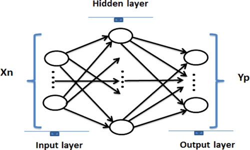
On this subject, we focus on the preparation of a DSS, to classify ECG recordings into normal and pathological class. Accordingly, three different feedforward ANNs, which are the Multilayer Perceptron (MLP) (Rafiq et al., 2001), the Radial Basic Function Network (RBF) (Zhao and Li, 2017), and the Probabilistic Neural Network (PNN) (Mao et al., 2000) are applied. We aim mostly to prepare the DSS to choose automatically the appropriate ANN structure, with respect to the users’ criteria. Consequently, while taking into account the accuracy (ACC), the time classification (Time_response), and the Mean Square Error (MSE), we have evaluated for each ANN, its optimum structure (MLP_opt, RBF_opt, and PNN_opt). Then, a comparative study between them is reached. After that, according to the demanded users’ criteria, the DSS chooses the appropriate optimum ANN structure.
This paper is organized as follows. In “Materials and methods” section, the proposed arrhythmia classification methodology is described. In this section, we begin by presenting the arrhythmia database MIT-BIH. Then, we present the feature extraction as well as the used feedforward artificial neural networks. Next, we detail the experiments and results in “Experiments and results” section. In “Discussion” section, a comparative study is discussed. Finally, a conclusion is reached.
Materials and methods
Overview
In order to prepare a DSS which classifies ECG signals into normal and abnormal class, we have followed the entire methodology described in the following block diagram (Figure 1). The block diagram includes two main stages which are Pre-processing and Neural Network arrhythmia classification. The first stage deals with the MIT-BIH ECG recordings pre-processing (Silva and Moody, 2014). In fact, Discrete Wavelet Transformer (DWT) coefficients and morphological features were extracted. Then, a correlation method is applied to select the most pertinent features. After that, the selected features are normalized and scaled to identify the input dataset. However, the second stage consists on the Neural Network Arrhythmia classification. This stage is based on the use of three feedforward ANN, as machine learning classifier, which are the MLP, the RBF, and the Probabilistic PNN.
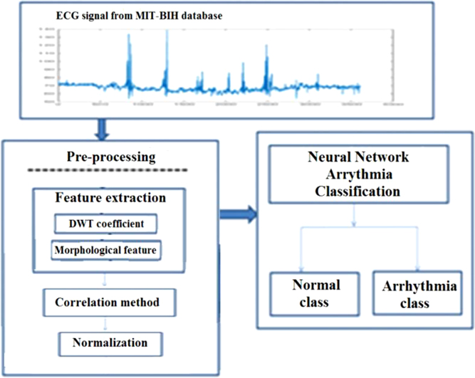
Figure 1
Block diagram of an ECG arrhythmia classification topic.
In this work, we focus mostly on the second stage. Therefore, according to the flow chart described in Figure 2, the input dataset is divided into two datasets used for training and testing the ANNs. The division respects the Association for the Advancement of Medical Instrumentation (AAMI) recommendations (De Chazel et al., 2004). In addition, according to Figure 2, structural and parametric studies are done in order to select the three optimum structures (MLP_opt, RBF_opt, and PNN_opt). Therefore, during these two studies, each ANN is trained and tested many times. Thus, several structures are obtained. Among them, the optimum one is which achieves the highest ACC, the fast Time_response, and the lowest MSE. But, when the obtained accuracies are equals, the ANN structure which has the fast Time_response is selected as the optimum one. Whereas, when both of the accuracies and time responses are equals, the optimum ANN structure is one which has the lowest MSE. After obtaining the optimum structures (MLP_opt, RBF_opt, and PNN_opt), a comparison study between them is investigated, according to the number of hidden neurons, ACC, Time_response, and MSE. Then, DSS chooses one of the optimum structures with respect to the users’ performance criteria. In fact, users might demand the DSS either to choose the ANN structure where decision time has got priority over decision accuracy, either to choose the most accurate ANN and no matter how rapid the network, or to choose automatically the structure without any requirements. In this case, the DSS chooses the most accurate network.
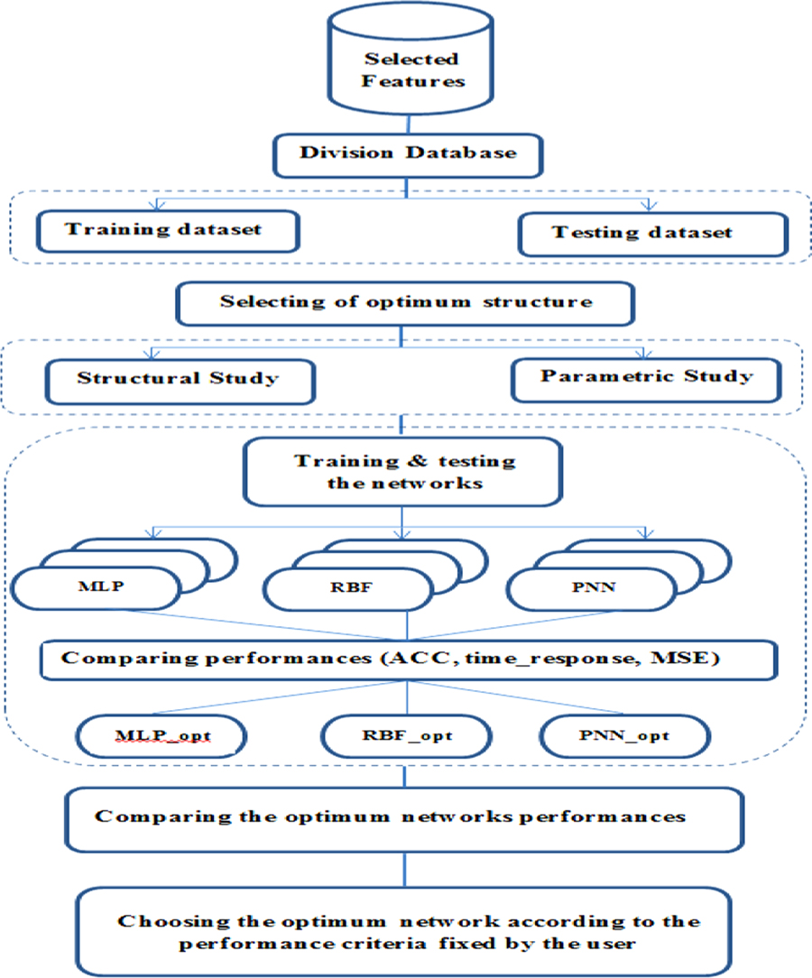
Figure 2
Flow chart of the proposed work.
The evaluation performances, used to evaluate the three ANNs, are described in the following equations:
where NCC is the number of correctly classified inputs vector, N is the number of inputs vector, Tr_time is the training time, and Test_time is the testing time.MITBIH arrhythmia database
The standard arrhythmia database MIT-BIH was used in this study. It contains 48 records of heartbeats at 360 Hz for approximately 30 min of 47 different patients. Each record has two ECG leads (lead A and lead B) which are depending on the electrodes configuration on the patient’s body. The database includes approximately 109,000 beat labels. In addition, it contains 25 normal records, 19 abnormal records, and 4 paced beats records (102, 104, 107, and 217) which were excluded in this study. Therefore, we have only treated the first minute of 44 ECG samples where those with arrhythmia can be interpreted as “1” and the other without arrhythmia can be interpreted as “0” (Silva and Moody, 2014).
Feature extraction
The classification stage of ECG waveforms requires the extraction of the corresponding features (Alfarhan et al., 2017). In fact, the ECG waveform, as it is shown in Figure 3, consists of three basic waves P, QRS, and T waves and sometimes U wave. Indeed, P wave arises due to the atrial depolarization, QRS complex represents the ventricular depolarization, and T wave arises due to the repolarization of the ventricle (De Chazel et al., 2004).
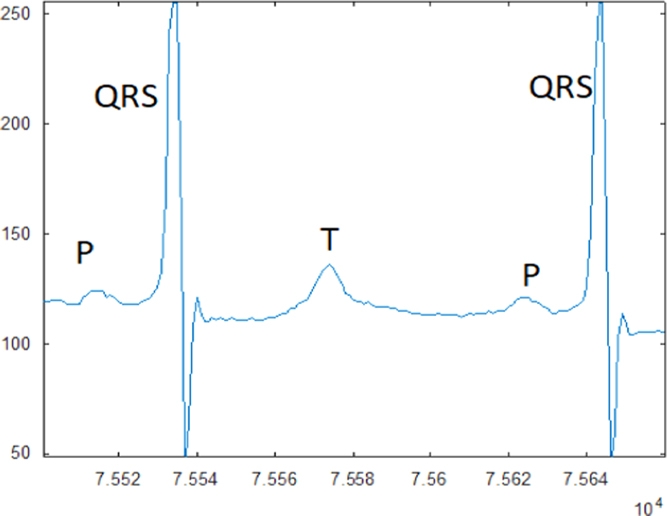
Figure 3
Normal ECG recording.
In this study, morphological and time frequency features are extracted (Lassoued and Ketata, 2017; Lassoued and Ketata, 2018). On the first hand, we have applied two MATLAB toolbox which are the waveform Database software Package (WFDB toolbox) (Silva and Moody, 2014) and the ECG-kit (Demski and Llamedo, 2016) to extract the morphological characteristics. Thus, we have identified for each ECG recording, peak values (P, Q, R, S and T), the standard deviation of time duration between waves (P-R, P-T, S-T, Q-T, Q-R-S, and R-R) and the mean and the standard deviation of the heart rate values (Lassoued and Ketata, 2017; Lassoued and Ketata, 2018). On the second hand, we have returned, for each ECG signal, the details and approximations coefficients of the discrete wavelet transformer (DWT) of the mother wavelet Daubechiesb6 (db6), with eight decompositions. Accordingly, we have considered their arithmetic mean, variance, and standard deviation. Finally, we have collected for each ECG record, a total of 62 features consisting of 48 DWT coefficients and 14 morphological characteristics (Lassoued and Ketata, 2017; Lassoued and Ketata, 2018).
Feature normalization
Although normalization is not necessary for MLP and RBF networks, it is recommended for PNN. So, for a fair comparison between the three different ANNs (MLP, RBF, and PNN), we have applied the WEKA Min-Max normalization function to standardize all features at the same level (Yadav et al., 2014; Jain et al., 2017), as it is shown in Equation (3). By applying this equation, all the component of the input feature vector are normalized and rescaled in the interval [0, 1]:
where Xmin and Xmax are the minimum and the maximum values for one feature, respectively. Xnor is the normalized feature vector and X is the original feature vector.Feature selection
The ACC of the classifier depends on several factors, such as the quality and the size of the input feature vectors. Thus, feature selection stage is required in order to use the most pertinent features and also to reduce the feature vectors size. For this purpose, we have applied the WEKA selection function “Correlation Attribute Eval” (Savic et al., 2017). This function evaluates features by measuring the correlation between the feature and the corresponding class (normal or abnormal). In this study, we have considered only the attributes having a correlation ranking up to 0.300. Therefore, the size of the input matrix becomes (10 × 44) instead of (62 × 44). Table 1 describes the degree of correlation for the 10 selected features.
Table 1
Selected attributes.
| Selected Features | Max-Q | Std-a6 | Std- a5 | Std- a7 | Std- a4 | Std- a3 | Std- a2 | Std-a1 | std- a8 | Moy-d8 |
|---|---|---|---|---|---|---|---|---|---|---|
| Correlation rank | 0.350 | 0.326 | 0.318 | 0.314 | 0.311 | 0.310 | 0.307 | 0.306 | 0.304 | 0.300 |
| Criteria types | Criterion | MLP | RBF | PNN | |||
|---|---|---|---|---|---|---|---|
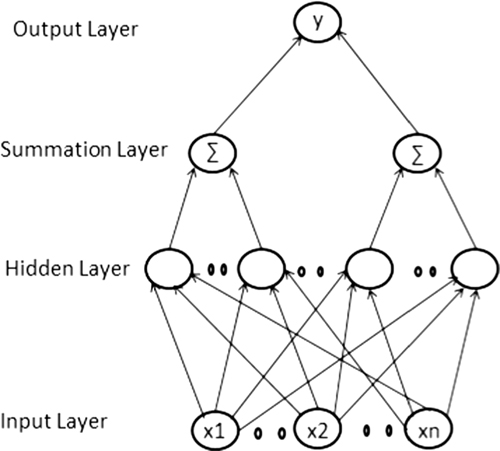
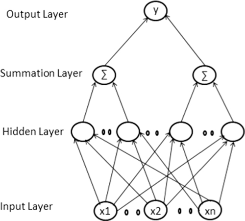
| Structural | Architecture | An input layer, one or more hidden layer and an output layer | An input layer, one hidden layer and an output layer | An input layer, one hidden layer, a summation layer and an output layer | |||
| Activation function | The activation function is non-linear (sigmoid, log-sigmoid, tan-sigmoid.) | The activation function is a radial basis function which computes the Euclidian distance of the input vector and its weights | The activation function is based on the probability density function | ||||
| Number of hidden neurons | no defined principle for determining the number of neurons | no defined principle for determining the number of neurons | The number is equal to the number of instance | ||||
| Output layer | The final layer uses the activation function before linearly combining it | The final layer doesn’t use activation function, it rather linearly combines the output of the previous neuron | The final layer is a competitive output layer. It picks the maximum of the computed probabilities | ||||
| Training Process | Backpropagation training algorithms | Backpropagation or clustering algorithms | There is no computation of weights. The Bayesian decision rule | ||||
| Parametric | Parameters | Momentum factor, learning rate, parameters according to the training algorithm | Number of centers, spread of radial function | Spread value of the probability density function | |||
| NO/HL | |||||||
|---|---|---|---|---|---|---|---|
| N_HL | H1 | H2 | ACC(%) | Tr_time(s) | Test_time(s) | Time_response (s) | MSE |
| 5 | 0 | 72.7 | 0.221 | 0.113 | 0.334 | 0.026 | |
| 10 | 0 | 86.4 | 0.222 | 0.094 | 0.316 | 0.024 | |
| 1 | 15 | 0 | 81.8 | 0.380 | 0.099 | 0.479 | 0.021 |
| 20 | 0 | 81.8 | 0.390 | 0.073 | 0.463 | 0.016 | |
| 25 | 0 | 81.8 | 0.406 | 0.071 | 0.477 | 0.013 | |
| 10 | 5 | 81.8 | 0.315 | 0.238 | 0.553 | 0.019 | |
| 2 | 10 | 10 | 81.8 | 0.319 | 0.253 | 0.572 | 0.021 |
| 10 | 15 | 72.7 | 0.383 | 0.281 | 0.664 | 0.018 | |
| 10 | 20 | 72.7 | 0.423 | 0.317 | 0.740 | 0.017 | |
| Learning algorithms types | Learning algorithms | ACC(%) | Tr_time(s) | Test_time(s) | Time_response (s) | MSE |
|---|---|---|---|---|---|---|
| Jacobian derivatives | trainlm | 86.4 | 0.222 | 0.024 | 0.246 | 0.094 |
| trainbr | 74.5 | 0.229 | 0.031 | 0.260 | 0.124 | |
| Gradient derivatives | trainscg | 86.4 | 0.553 | 0.355 | 0.908 | 0.077 |
| traingda | 81.8 | 0.416 | 0.218 | 0.634 | 0.078 | |
| trainrp | 86.4 | 0.294 | 0.096 | 0.390 | 0.073 | |
| traingdx | 81.8 | 0.543 | 0.345 | 0.888 | 0.076 | |
| trainbfg | 86.4 | 0.330 | 0.132 | 0.462 | 0.087 | |
| traincgb | 81.8 | 0.316 | 0.118 | 0.434 | 0.070 |
| Lr | ACC(%) | Time_response (s) | MSE | |||
|---|---|---|---|---|---|---|
| 0.01 | 86.4 | 0.390 | 0.130 | |||
| 0.1 | 86.4 | 0.399 | 0.064 | |||
| 1 | 86.4 | 0.392 | 0.073 |
| NO/HL | ACC (%) | Tr_time(s) | Test_time(s) | Time_response (s) | MSE | |
|---|---|---|---|---|---|---|
| 5 | 54.5 | 0.380 | 0.015 | 0.395 | 0.204 | |
| 10 | 59.1 | 0.436 | 0.013 | 0.449 | 0.150 | |
| 15 | 81.8 | 0.501 | 0.014 | 0.515 | 0.080 | |
| 20 | 99.9 | 0.640 | 0.014 | 0.654 | 1.266e-30 | |
| 25 | 99.9 | 0.699 | 0.017 | 0.716 | 2.411e-30 |
| RBF functions | ACC(%) | Tr_time(s) | Test_time(s) | Time_response (s) | MSE | |
|---|---|---|---|---|---|---|
| Gaussian | 99.9 | 0.380 | 0.014 | 0.654 | 1.266e-30 | |
| Polyharmonic | 99.9 | 0.436 | 0.051 | 0.639 | 1.221e-30 | |
| Inverse_multiquadric | 99.9 | 0.501 | 0.121 | 0.676 | 0.250e-30 | |
| Multiquadric | 99.9 | 0.640 | 0.132 | 0.698 | 0.891e-30 | |
| Biharmonic | 99.9 | 0.699 | 0.002 | 0.640 | 0.891e-30 |
| Basic function | Spread | ACC(%) | Test_time(s) | Time_response (s) | MSE | |
|---|---|---|---|---|---|---|
| Inverse_multiquadric | 10 | 99.9 | 0.121 | 0.643 | 0.250 e-30 | |
| 1 | 99.9 | 0.128 | 0.668 | 0.250 e-30 | ||
| 0.1 | 99.9 | 0.140 | 0.676 | 0.250 e-30 |
| NO/HL | ACC(%) | Tr_time(s) | Test_time(s) | Time_response (s) | MSE | |
|---|---|---|---|---|---|---|
| 22 | 79.5 | 0.081 | 0.218 | 0.299 | 0.162 |
| Spread | ACC(%) | Test_time(s) | Time_response (s) | MSE | ||
|---|---|---|---|---|---|---|
| 0.1 | 79.5 | 0.081 | 0.218 | 0.162 | ||
| 1 | 79.5 | 0.070 | 0.218 | 0.162 | ||
| 10 | 79.5 | 0.074 | 0.218 | 0.162 |
| ANN | N0/HL | ACC(%) | Tr_time(s) | Test_time(s) | Time_response (s) | MSE |
|---|---|---|---|---|---|---|
| MLP_opt | 10 | 86.4 | 0.294 | 0.096 | 0.390 | 0.064 |
| RBF_opt | 20 | 99.9 | 0.755 | 0.121 | 0.876 | 0.250 e-30 |
| PNN_opt | 22 | 79.5 | 0.070 | 0.218 | 0.288 | 0.162 |
| ANN | Pre-processing | Test conditions | Division Datasets | ACC(%) |
|---|---|---|---|---|
| (Abhinav-Vishwa et al., 2011) | R peak | MIT_BIH database of 48 signals of 30 min | 50% for training and 50% for testing | 96.8 |
| (Rai et al., 2013) | Morphological and DWT coefficients | 45 ECG signal of 1 min from MIT-BIH database | 26 signals for training and 19 for testing | 97.8 |
| (Tomar et al., 2013) | Morphological, DWT coefficients, power spectral density and Energy of Periodogram | 62 ECG signals of 10 s from MIT-BIH database and Normal Sinus Rhythm (NSR) | Cross validation division (70%, 30%) | 98.4 |
| (Savalia et al., 2017) | R peaks, the heart beats/min, the duration of complex QRS | 66 ECG signal from MIT_BIH arrhythmia database and NSR database | Cross validation division (70%, 30%). | 82.5 |
| (Dalvi et al., 2016) | QRS complex, RR interval and the beat waveform morphology. PCA for feature selection | MIT_BIH database of 48 signals of 30 min. | 18 ECG records for test dataset and 30 ECG for train dataset | 96.9 |
| Proposed work | Morphological and DWT coefficients | 44 ECG signals of 1 min. recording from MIT_BIH database | 22 signal for training and 22 for testing following the AAM.I recommendations | 99.9 |