I. INTRODUCTION
Increasing demands and progressive development process have compromised sustainability potential of the coastal lakes in Egypt. The quality of water resources dictates beneficial uses offered as well as functionality of the aquatic ecosystem, especially with the alarming pollution level associated with the anthropogenic activities. Thus, continuous monitoring and frequent update of water resources status are required for sound management planning and corrective measure scenarios. However, such tasks require comprehensive data collection with adequate temporal and spatial coverage. Remote sensing is an advancing field that has the potential in reducing field work difficulties, and increasingly considered an essential planning tool.
A. Remote Sensing-based Water Quality Retrieval
Several studies in literature have addressed retrieval of water quality parameters using remote sensing techniques. Significant correlations have been found between specific water quality parameters and reflectance measured with satellite sensors. These parameters cause change to the spectral properties of reflected light and, hence, are remotely detectable (Gholizadeh et al., 2016). Recent research by Swain and Sahoo (2017) argued that certain conservative pollutants can be distinctively detected with different reflectance received in the electromagnetic spectrum because no biochemical reactions or ionic exchange are experienced.
Retrieving properties such as water clarity; turbidity, and Total Suspended Solids (TSS) concentrations using earth observation imageries have been tackled in applied research studies worldwide (Kloiber et al. 2002; Zhang, 2002; Bilge et al., 2003; He et al., 2008; Sravanthi et al., 2013; Dona et al., 2014; Dorji and Fearns 2016; Abayazid and El-Gamal 2017). In 2008, He et al. presented water quality retrieval models with proven successful results for optical nitrogenous and phosphorous components. Other parameters such as chlorophyll-a (chl-a) and Colored Dissolved Organic Matter (CDOM)) have also been covered in various studies (i.e. Brezonik et al., 2005; Thiemann and Kaufmann, 2000; Li et al., 2002; Dona et al., 2014).
Remotely deriving weak and/or non- optical water quality characteristics, that have no directly-detectable reflection, is challenging. Consequently, early studies are mostly focused on water physical and biogeochemical components that are considered optically active (Giardino et al., 2014). However, limitation to water quality characteristics that are related to Inherent Optical Property (IOP) narrows down the parameters that can be assessed by remote sensing techniques.
The Dissolved Oxygen (DO) concentration is considered a crucial indicator of water system healthiness, and governs recovery capability (UNESCO, 2005). Yet, being a non-optically active parameter, DO levels cannot be directly retrieved using remote sensing technique. This research study aims to present an approach to detect Dissolved Oxygen concentrations in an inland shallow coastal lake, using space-based imageries.
Based on grounds of early DO modeling theories, as well as regional conditions, the study investigates the potentiality of deducing DO levels from optically detectable water quality parameters that affect, and be affected by, Oxygen presences in water.
B. Study Area
With growing population and development activities, the Nile Delta of Egypt experience challenging conditions. Lake Edku is located within the active Northwestern coastal zone of the Delta, between longitudes 30°8’ & 30°23’E and latitudes 31°10’ & 31°18’N (Fig. 1). The lake is characterized of having systematically shrinking free open water, altered ecosystem and deteriorating water quality state (Abayazid, 2015). Edku lake serves an active agriurban basin, and bordered by dense aquaculture practices. Accordingly, the lake receives wastewaters with different pollution degree from fish farming therapeutic drugs, nutrient flux from agricultural drainage network (e.g. Edku, El-Boussili, Khairy and Bearsik drains), in addition to effluents from municipal WasteWater Treatment Plants (WWTPs) and industrial facilities (Siam and Ghobrial, 2000). The lake is connected to the Mediterranean Sea with single opening “Boghaz Al-Maadia”, which allows temporal tidal inflows and localized saline water interaction. Discharges with heavy nutrient levels, as well as the deceased salinity inputs, have encouraged excessive unwanted aquatic vegetation. That, in turn, disturbed natural circulation; flow dynamic and sediment transport, and hence self –purification within the lake (Hossen and Negm, 2017).
II. MATERIALS AND METHODS
This section addresses the basis of DO modeling that dictated selection process to the parameters included in this study application. Also, the ground truth data and corresponding satellite imageries considered are presented, and then followed by the approach adopted for algorithm development.
A. Theory: Grounds for DO Modeling
Modeling of Dissolved Oxygen in water bodies has been initiated in 1925 by Streeter and Phelps through an application in the Ohio River of the United States of America (Chapra, 1997). Simulation studies were based on the fact that the rate at which DO fluctuates in waters reflect the rate of Oxygen demand and release. Their modified model set foundation of DO sinks and sources through inclusion of factors proved affecting the Dissolved Oxygen depletion and recovery in a water body. Beside the initially considered coefficients that represent reaeration as well as settling/ decay processes, the model extension added representative components of aquatic flora role in the Oxygen production and exhaustion with photosynthetic activity. Furthermore, sediment consumption of DO has been added as an effective factor to be employed in the modified model for DO prediction. Equations 1 and 2 state the early model and modefied version; respectively. More details can be found in the text book of Chapra (1997)
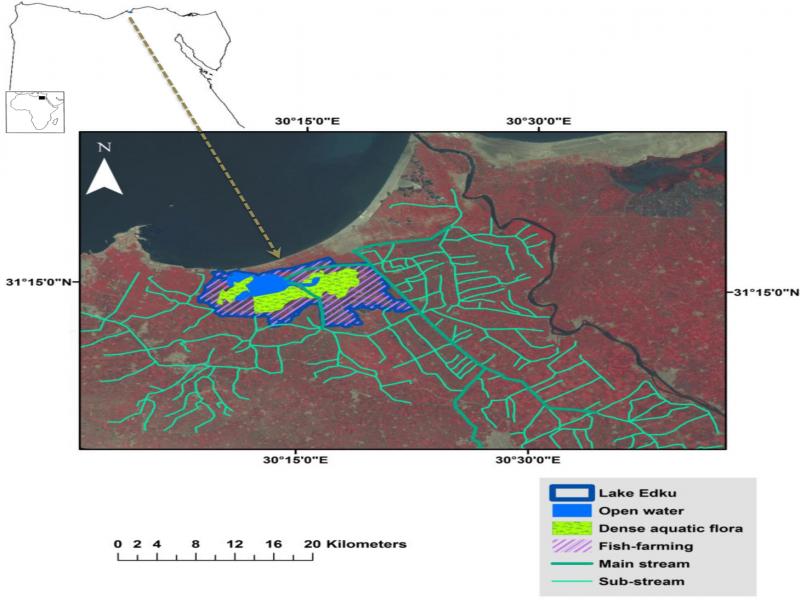
Figure 1.
Edku Lake
Where; Dt is the predicted dissolved oxygen deficit concentration, t is the travel time, L is the BOD level at point of interest, Lo is the ultimate BOD level, Ka is the reaeration rate, Kd is the decomposition rate, Ks is the settling removal rate, Kc is the CBOD decay coefficient, and Do is the initial value of the oxygen deficit.
The modified model has added factors as; P the photosynthetic oxygen production rate, R the algal respiration rate, Sb the sediment oxygen demand rate, No the initial Nitrogenous BOD (NBOD), and Kn the NBOD decay coefficient.
B. Field Measurements
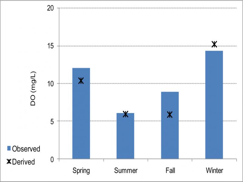
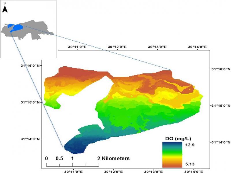
Ground truth data used were obtained from published research study by Okbah et al. (2017). Authors presented data collected in ten sampling locations distributed throughout the Edku Lake. Spatial distribution of field measurement locations reflects variability in the lake water quality, with regard to boundary interaction as well as flow movements within the lake (Fig. 2). Further, sampling campaigns have been carried out during four seasons; spring, summer, fall and winter of year 2016, which reflected the variable conditions that the coastal lake experince. Statistics of the field measurements show that in summer time DO levels reach the lowest concentrations, ranging from 1.6 to 9.4 mg/L, and experience wide variability within the lake with standard deviation of 3 among the ten investigated locations. Meanwhile, the highest DO levels occur in winter, ranging from11.3 to 18.1 mg/L, with standard deviation of 2.3. The lake water DO range from 7.5 to 14.0 mg/L in spring, whereas the fall season has slightly less concentrations, ranging from 5.0 to 13.1 mg/L. Maximum measured DO concentrations were mostly found in zones “C” and “D”, as illustrated in figure (3). On the other hand, minimum levels occur in locations within the eastern zone “A”, where most of direct wastewater discharges reach the lake water, especially in summer season.
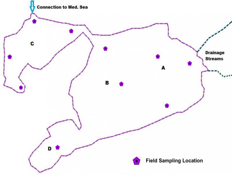
Figure 2.
Field measurement locations in Lake Edku zones A, B, C, and D
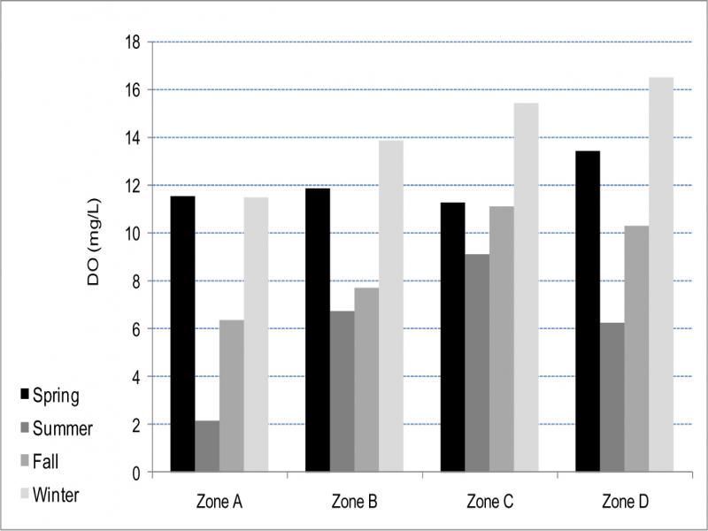
Figure 3.
Observed DO data during four seasons in Lake Edku zones
C. Remote Sensing Data
In 2013, Ganoe and DeYoung presented theoretical basis for DO retrieval with the use of air-borne Raman spectroscopy instead of ship-based technology that customary required direct contact with the waterbody. Authors argued the advantages of air-based technique in measuring DO when compared to time consuming as well as limitation in detecting variability in changing water conditions during field trips. The research concluded promising success of remote sensing retrieval of the temporal and spatial dynamics of dissolved gas distributions in coastal ecosystems. Yet aerial arrangements are costly and not always readily available, while space-borne sensors can have more frequent revisits and reasonably spatial coverage with advancing spectral resolution.
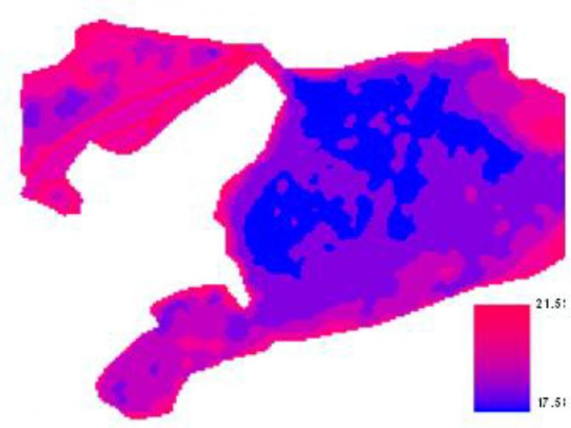
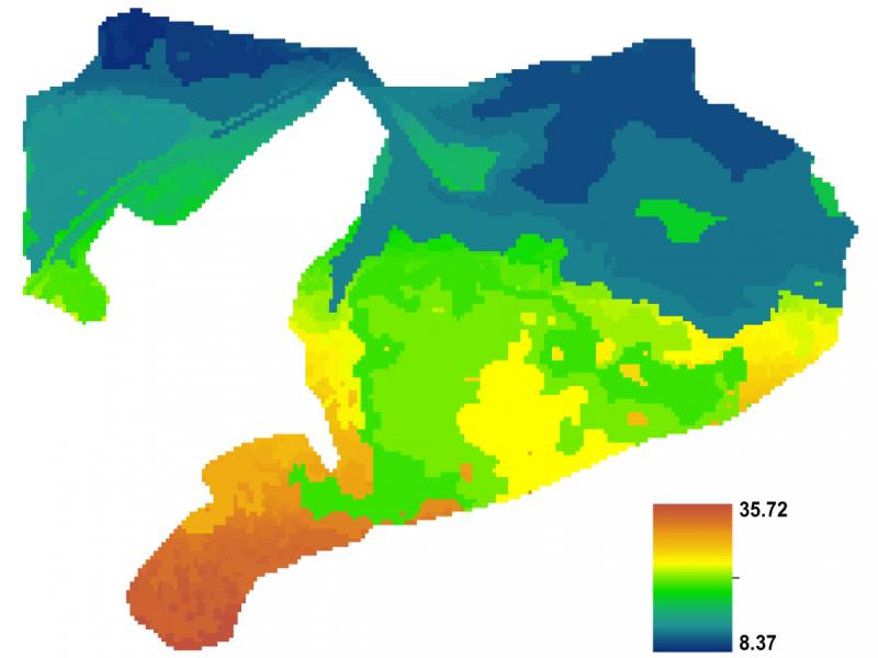
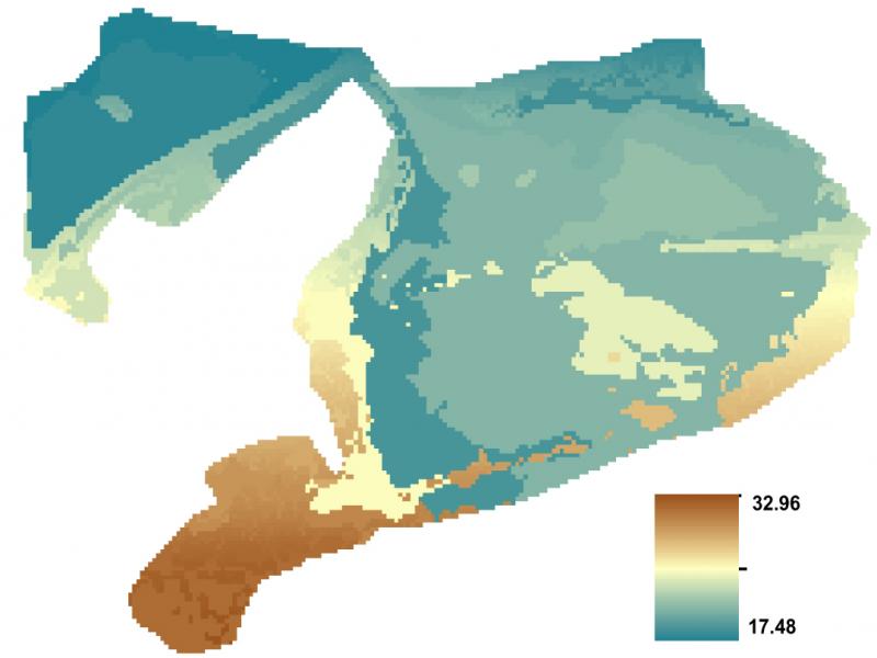
The imageries used in this study are the freely available Landsat 8 Operational Land Imager (OLI) from the Unitd States Geological Survey (USGS) Earth- Explorer website. The Landsat 8 (OLI/TIRS) is the most recent satellite that was launched in 2013 under the Landsat program, with swath width of 170 km and 16 days’ revisit interval. Since the in situ DO data have been collected during spring, summer, fall and winter of year 2016, images used in this study were acquired on nearest corresponding overpass dates to match the sampling data timing Table (1). Table (2) states the spectral range considered in this study, covering visible and Near-Infrared as well as Thermal Infrared bands. The necessary image processing and result analysis were carries out in Geographic Information System (GIS) environment.
TABLE I.
USED LANDSAT 8 (OLI) SCENES AND DATES OF ACQUISITION
| Scene ID (path177/row38) | Date Acquired | |
|---|---|---|
| “LC81770382016071LGN01” | 11-Mar-2016 | |
| “LC81770382016151LGN01” | 30-May-2016 | |
| “LC81770382016231LGN01” | 18-Aug-2016 | |
| “LC81770382016343LGN01” | 8-Dec-2016 | |
| Landsat 8 (OLI) bands | Spectral range (μm) | |
|---|---|---|
| Band 2 (Visible) | 0.450 - 0.51 | |
| Band 3 (Visible) | 0.53 - 0.59 | |
| Band 4 (Visible) | 0.64 - 0.67 | |
| Band 5 (Near-Infrared) | 0.85 - 0.88 | |
| Thermal Infrared Sensor (TIRS) | ||
| Thermal Infrared (Band 10) | 10.6 - 11.19 | |
| Thermal Infrared (Band 11) | 11.5 - 12.51 | |
| Seasons | Input Parameters | Regression Coefficient (R2) |
|---|---|---|
| Spring & Fall & Winter | Turb, TSS, Chl, Ln-temp | 0.618 |
| Summer & Fall & Winter | Turb, TSS, Chl, Ln-temp | 0.630 |
| Spring & Summer & Fall | Turb, TSS, Chl, Ln-temp | 0.657 |
| Summer & Fall | Turb, TSS, Chl, Ln-temp | 0.781 |
| Spring & Fall | Turb, TSS, Chl, Ln-temp | 0.751 |
| Spring & Winter | Turb, TSS, Chl, Ln-temp | 0.651 |
| Spring & Summer & Fall | Turb, TSS, Ln-temp | 0.613 |
| Summer & Fall & Winter | Turb, TSS, Ln-temp | 0.601 |
| Spring & Fall & Winter | Turb, TSS, Ln-temp | 0.584 |
| Spring & Fall | Turb, TSS, Chl | 0.644 |
| Spring & Fall | TSS, Chl, Ln-temp | 0.676 |
| Spring & Winter | TSS, Chl, Ln-temp | 0.554 |
| Summer & Fall | Turb, TSS, Ln-temp | 0.766 |
| Summer & Fall | Turb, Chl, Ln-temp | 0.798 |
| Summer & Fall | TSS, Ln-temp | 0.756 |
| Summer & Fall | Turb, Ln-temp | 0.792 |
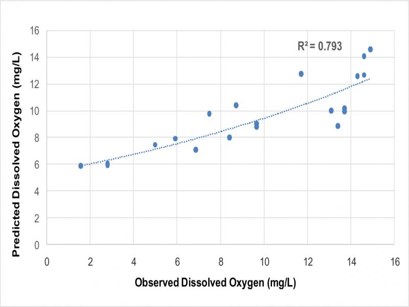
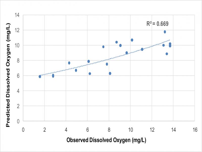
| Descriptive Statistics | Do (mg/L) | |
|---|---|---|
| Observed | Modeled | |
| Mean | 10.440 | 9.064 |
| Minimum | 1.560 | 4.552 |
| Maximum | 18.107 | 20.271 |
| Standard Deviation | 4.042 | 3.841 |