
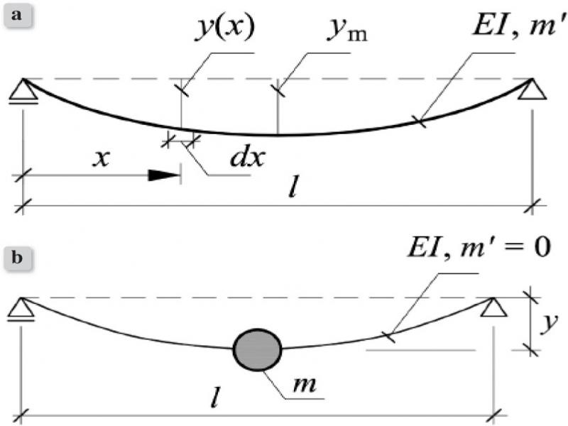
Figure 1.
Reduction of the beam with the continuous distribution of mass into the system with one degree of freedom a) system with the continuous distribution of mass m′, b) substitute mass m lumped in the point in which the arrow of vibrations of the system with continuous distribution of mass occurs
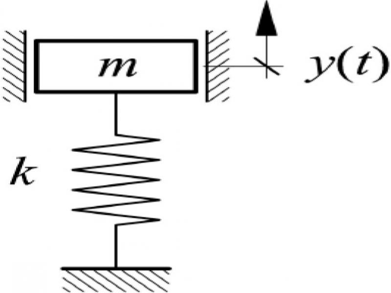
Figure 2.
Oscillator of parameters k and m as the substitute system for the reinforced concrete beam
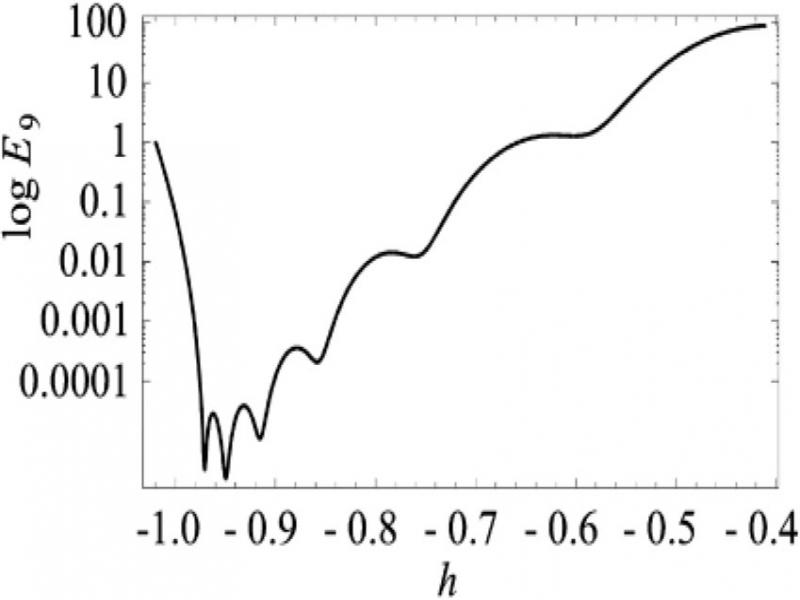
Figure 3.
The squared residual E 9
Table 1.
Values of errors in the reconstruction of the exact solution (Δ n = ||ye – ŷn ||)
| n | 1 | 2 | 3 | 4 | 5 |
|---|---|---|---|---|---|
| Δ n | 0.187 | 0.390 | 0.287 | 0.101 | 1.767·10-2 |
| n | 6 | 7 | 8 | 9 | 10 |
| Δ n | 1.187·10-3 | 4.884·10-5 | 7.253·10-6 | 3.744·10-7 | 2.572·10-8 |
| n | 11 | 12 | 13 | 14 | 15 |
| Δ n | 3.130·10-9 | 8.340·10-11 | 1.165·1-11 | 1.101·10-12 | 3.706·10-14 |
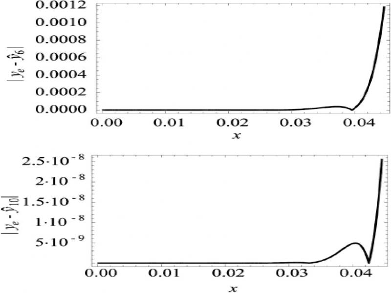
Figure 4.
Distribution of error (|ye (x) – ŷn (x)|) of the exact solution approximation for n = 6 (a) and n = 10 (b)
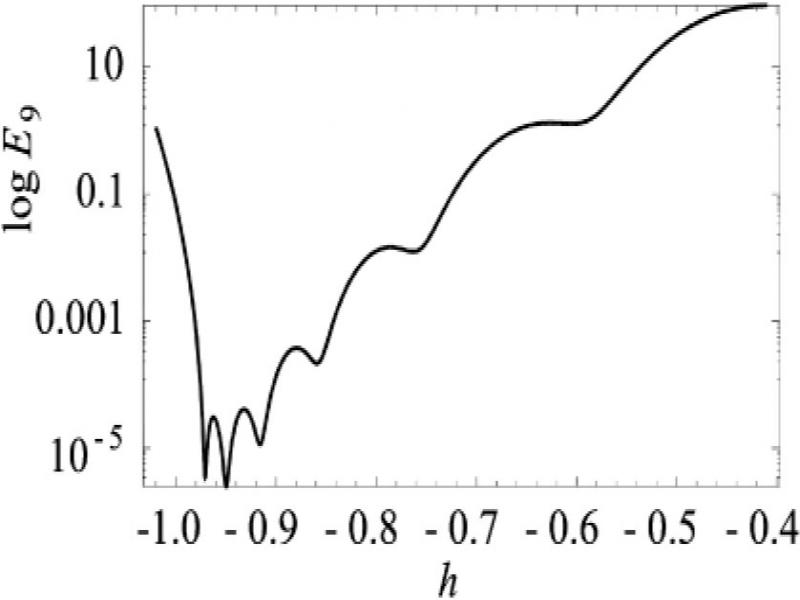
Figure 5.
The squared residual E 9
Table 2.
Values of errors in the reconstruction of the exact solution (Δ n = ||ye – ŷn ||)
| n | 1 | 2 | 3 | 4 | 5 |
|---|---|---|---|---|---|
| Δ n | 0.236 | 0.456 | 0.333 | 0.122 | 2.388·10-2 |
| n | 6 | 7 | 8 | 9 | 10 |
| Δ n | 2.283·10-3 | 4.017·10-5 | 8.665·10-6 | 8.046·10-8 | 3.744·10-8 |
| n | 11 | 12 | 13 | 14 | 15 |
| Δ n | 7.420·10-10 | 1.238·10-10 | 7.527·10-12 | 1.437·10-13 | 2.802·10-14 |
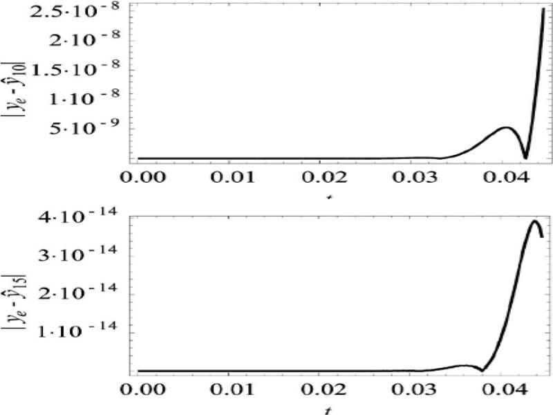
Figure 6.
Distribution of error (|ye (x) – ŷn (x)|) of the exact solution approximation for n=10 (a) and n=15 (b)
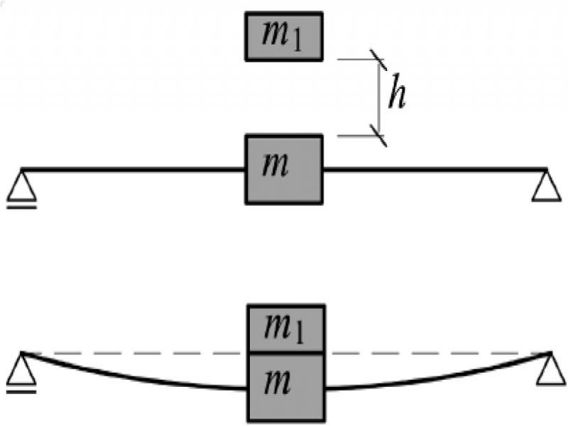
Figure 7.
Impact of plastic character implying the initial conditions y(0)=0 and ẏ (0)=va (a, b – described in text)
Table 3.
Values of errors in the reconstruction of the exact solution (Δ n = ||ye – ŷn ||)
| n | 1 | 2 | 3 | 4 | 5 |
|---|---|---|---|---|---|
| Δ n | 3.367·10-2 | 2.084·10-2 | 1.741·10-3 | 1.374·10-3 | 4.188·10-4 |
| n | 6 | 7 | 8 | 9 | 10 |
| Δ n | 5.135·10-5 | 1.785·10-5 | 9.227·10-5 | 2.483·10-6 | 4.230·10-7 |
| n | 11 | 12 | 13 | 14 | 15 |
| Δ n | 6.678·10-8 | 2.612·10-8 | 1.181·10-8 | 3.571·10-9 | 8.398·10-10 |
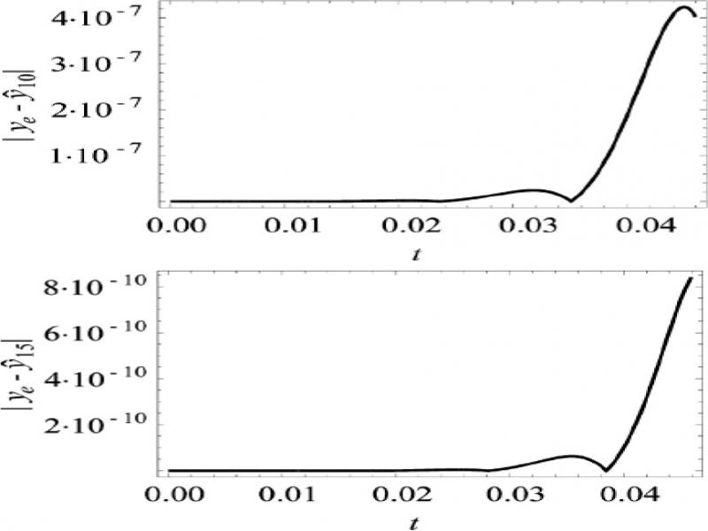
Figure 8.
Distribution of error (|ye (x) – ŷn (x)|) of the exact solution approximation for n=10 (a) and n=15 (b)
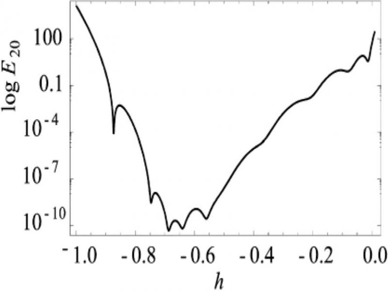
Figure 9.
The squared residual E 20
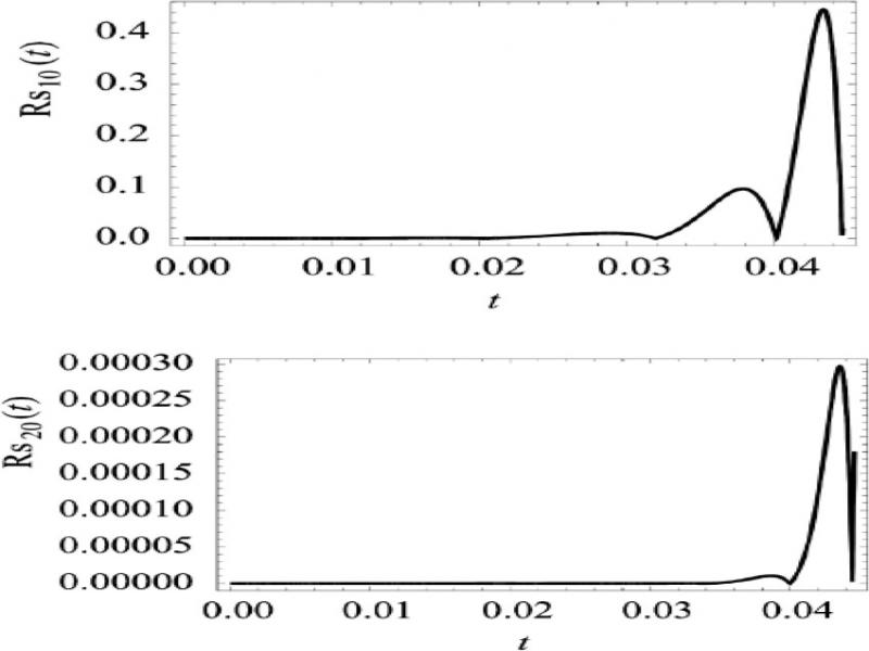
Figure 10.
Plot of the residual Rsn for n=10 (a) and n=20 (b)
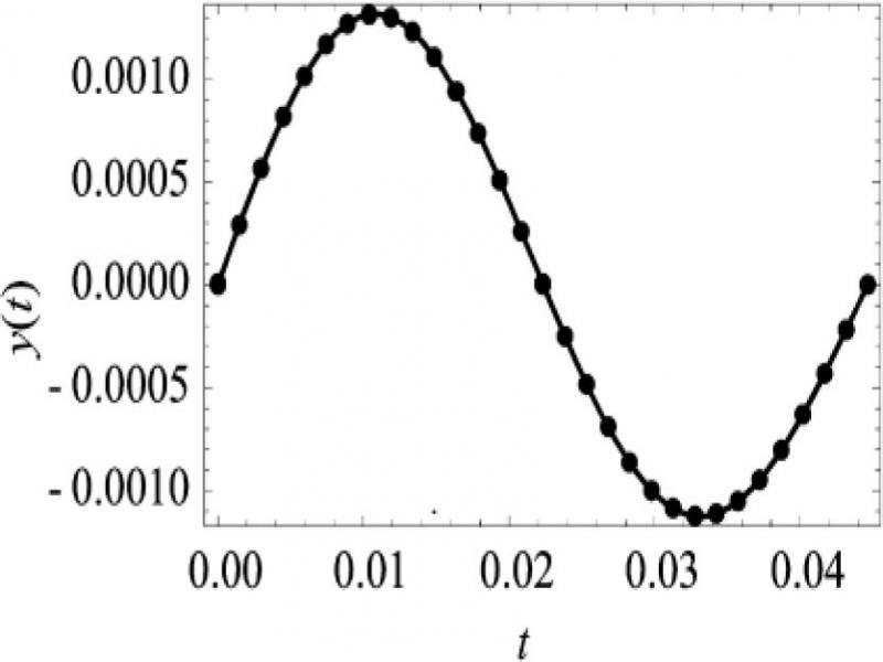
Figure 11.
Comparison of the approximate solutions (solid line – solution ŷ20 obtained by the homotopy analysis method, dots – approximate solution obtained numerically in Mathematica software)
Table 4.
Maximal absolute differences (Δ n ) between the approximate solutions obtained by the homotopy analysis method and the numerical methods available in Mathematica software
| n | 1 | 3 | 5 |
|---|---|---|---|
| Δ n | 3.35·10-2 | 4.98·10-3 | 7.12·10-5 |
| n | 10 | 15 | 20 |
| Δ n | 1.40·10-6 | 2.99·10-8 | 3.71·10-9 |
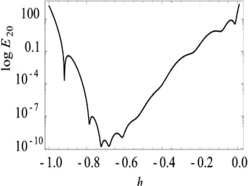
Figure 12.
The squared residual E 20
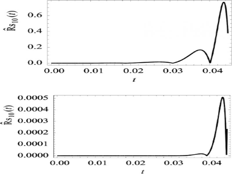
Figure 13.
Plot of the residual for n=10 (a) and n=20 (b)
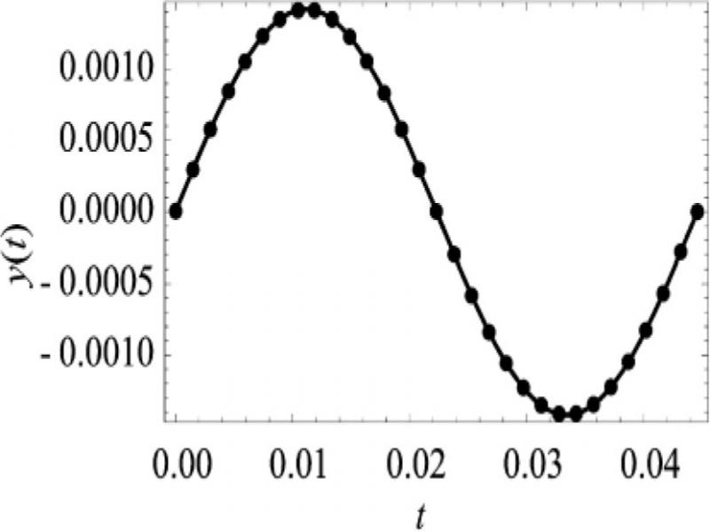
Figure 14.
Comparison of the approximate solutions (solid line – solution ŷ20 obtained by the homotopy analysis method, dots – approximate solution obtained by the numerical method available in Mathematica software)