Access to credit (direct or indirect finance, formal or informal credit) is viewed as one strategy for increasing agricultural productivity. Farmers’ improved access to credit has been linked to increased use of agricultural inputs, increased technical efficiency, and widespread adoption of cutting-edge technology (Wanzala et al., 2024). As a result of persistently limited access to the levels of credit that would allow smallholder farmers to acquire the optimal quantity of production components, most developing countries’ economic development is hampered. For example, the real GDP growth rate of Kenya’s agriculture sector (AS) was 5.3% in 2015, 4.7% in 2016, and 1.9% in 2017. According to the Central Bank of Kenya (2019), the AS real GDP growth rate of 6.4% in 2018 was accompanied by a deterioration in quarterly growth, with 7.5%, 6.5%, 6.9%, and 3.9% for the first, second, third, and fourth quarters, respectively. Coffee production is an agricultural sector plagued by limited access to credit, resulting in consistently poor performance (ICO, 2019). Coffee was regarded as Kenya’s black gold until 1989, owing to its significant contribution to GDP. Despite this, coffee exports fell from 40% of total exports in 1985 to 0.42% in 2019 (Wanzala et al., 2022). Although the coffee sector’s poor performance may not be directly related to a lack of credit, policymakers and researchers believe that an in-depth examination should be conducted as soon as possible to determine what is wrong with the sector.
Above all, the GoK recognizes that to successfully stimulate rural development and alleviate poverty, the government must consistently work to create an enabling environment for credit availability in order to promote agricultural productivity (Wanzala et al., 2021). However, many rural communities in Kenya have weak or non-existent official financial institutions, making it difficult to provide adequate agricultural financing (Lydia et al., 2023). Furthermore, asymmetric information and moral hazard have caused credit market flaws, resulting in credit rationing (Stiglitz and Weiss, 1981) and a drop in agricultural productivity. For example, in 2015, the loan requirements of the key agricultural commodity value chain were estimated to be US$ 1,300 million, but the agricultural sector had a loan deficit of US$ 900 million (World Bank, 2018). This is despite the Kenyan government’s establishment of the Commodity Fund (formerly known as the Coffee Development Fund) in 2006 to address the market’s failure to provide farmers with long-term and affordable agricultural financing (Wanzala et al., 2024). The collateral requirement is optional, but smallholder farmers must be members of a specific coffee association or coffee farmers’ cooperative society.
The Commodity Fund, in particular, was established to boost coffee production, alleviate poverty, and foster economic development. Nevertheless, Kenya has shown consistent declines in coffee productivity from 2007 to the present (Wanzala et al., 2022). Similarly, despite GoK engagement, loan acceptance remains low; for example, agricultural credit accounted for only 4.3% of total private sector credit in 2016 (World Bank, 2018). Furthermore, according to Central Bank of Kenya (2019) data, agricultural credit accounted for 3.62 percent of total credit in 2018, as shown in Table 1. According to FinAccess (2019), a sizable proportion of smallholder farmers finance agricultural output through limited savings, credit from well-wishers (family, relatives, and friends), loan sharks, and self-help organizations.
Sectoral loan topology: No. of loan A/Cs, gross loans and NPLs-December 2018
| No of loan A/Cs | % of total | Gross loans KShs. M | % of total | Gross NPLs KShs. M | % of total | |
|---|---|---|---|---|---|---|
| Personal/household | 6,728,258 | 93.63 | 661,460 | 26.63 | 45,672 | 14.42 |
| Trade | 255,409 | 3.55 | 475,423 | 19.14 | 81,622 | 25.77 |
| Real estate | 28,050 | 0.39 | 376,237 | 15.15 | 47,033 | 14.85 |
| Manufacturing | 15,213 | 0.21 | 323,817 | 13.04 | 51,791 | 16.35 |
| Transport and communication | 30,455 | 0.42 | 164,271 | 6.61 | 14,674 | 4.63 |
| Energy and water | 2,186 | 0.03 | 109,613 | 4.41 | 6,859 | 2.17 |
| Building and construction | 10,559 | 0.15 | 102,837 | 4.14 | 23,692 | 7.48 |
| Financial services | 14,986 | 0.21 | 95,780 | 3.86 | 6,049 | 1.91 |
| Agriculture | 95,158 | 1.32 | 89,961 | 3.62 | 30,452 | 9.62 |
| Tourism, restaurant and hotels | 4,548 | 0.06 | 72,134 | 2.9 | 6,392 | 2.02 |
| Mining and quarrying | 1,143 | 0.02 | 11,987 | 0.48 | 2,478 | 0.78 |
| Total | 7,185,965 | 100 | 2,483,518 | 100 | 316,712 | 100 |
Note: No. of loan A/Cs is number of loan accounts; KShs. M is million Kenya shillings; NPLs is non-performing loans.
Source: Central Bank of Kenya, 2019 (Bank Supervision, page 35).
The low acceptance of agricultural financing raises the question: do farmers’ views of credit undermine coffee productivity and thereby shape the current depressing trend in coffee production? Do they impede the GoK’s policy goal of increasing coffee productivity and transforming farmer livelihoods? To answer these questions, a more in-depth examination of the phenomenon of dismal performance in coffee production is required, which appears to contradict the conventional economic paradigm (Frankfurter and McGoun, 2018). In particular, it is necessary to investigate how farmers perceive the link between agricultural loans and coffee productivity.
Previous research on the relationship between credit and coffee productivity has yielded conflicting results. Some studies have discovered a strong positive relationship between credit and farm productivity (Diallo et al., 2020; Agbodji and Johnson, 2021; Rivera-Acosta and Xiuchuan, 2023), while others have found a negative relationship (Ashok et al., 2020; Bidishaa et al., 2018; Nakano and Magezi, 2020). Nonetheless, several studies have discovered a weakly positive, ambiguous, or insignificant link between credit and agricultural output (Khan et al., 2013; Njeru et al., 2016). This study differs from previous research by using both qualitative and quantitative methods, whereas previous studies primarily used quantitative techniques. Furthermore, there have been few studies on how people perceive the impact of credit on agricultural productivity. Existing research focuses on investor behavior in the stock market, credit perception, and other variables besides agricultural productivity (Bossaerts et al., 2019; Al-Zahrani et al., 2019). As a result, this study compares and contrasts farmers’ and investors’ perspectives on the impact of financing on coffee productivity.
The theoretical review for this study is based on rational economic theories (RET) and bounded rationality theories (BRT), which have played an important role in economics since the beginning of the twentieth century (Vriend, 1996). The specific theories considered for RET include expected utility theory (EUT), subjective expected utility theory (SEUT), and prospect theory (PT). From the perspective of RET economics, this study assumes that smallholder coffee farmers are rational and risk-averse. This means they have the ability and motivation to objectively weigh all available credit options from various market sources and select the one that maximizes coffee output. Furthermore, it is assumed that the credit source chosen will reduce losses, inefficiencies, and risks. Nonetheless, this theory assumes that farmers have access to all credit-related information and can use it to make informed decisions that increase coffee productivity. In fact, whether or not they secure credit to acquire production input and maximize output is determined by their perception of the credit’s impact on coffee output and returns (Arrow, 1982).
The EUT is a set of assumptions against which observations of actual decision-making can be compared (von Neumann and Morgenstern, 1947). Making a rational decision entails making a preference-free assessment of the available options before selecting a clear alternative based on the expected outcome. Farmers making decisions are assumed to be reliably capable of selecting an alternative based on all available information and to be unconcerned about how alternatives are presented. Bernoulli (1954) presented the marginal utility function (MUF) in the 18th century, providing a foundation for accepting that utility varies between people. This is consistent with Subjective Expected Utility Theory (SEUT), which states that people with different utility functions and beliefs about outcomes may make different decisions (Savage, 1954). In classical economics, utility is defined as the degree of satisfaction that an individual derives from the consumption of goods or services. Thus, obtaining credit from this perspective would entail an assessment of utility in terms of coffee production. For example, would using agricultural credit to purchase production inputs (seedlings, fertilizers, agrochemicals, and labor, among other things) increase utility or maximize coffee output?
Farmers in the rural credit market face three types of credit constraints: price rationing, credit rationing, and risk rationing. Price rationing occurs when credit is not cost-effective because the borrowing costs exceed the expected returns. Price rationing is typically caused by government intervention in the credit market through various strategies (Besley, 1994). For example, the government enacts laws requiring commercial banks to reserve a portion of their loan portfolio for farmers, and the government subsidizes loans through established state-owned banks. Such efforts will be futile if the farmers perceive the intended credit to have no significant implicit value to them in one way or another. Perhaps this is why, despite the government’s efforts to promote lending to small-scale farmers, farmers borrowed heavily from the informal sector (59%) as opposed to the GoK and formal sectors (1.3% and 22.7%, respectively) between 2010 and 2020. Credit rationing, on the other hand, describes a situation in which credit is profitable but lenders are unable to obtain desired amounts of credit at the equilibrium interest rate (Stiglitz and Weiss, 1981; Ghosh et al., 1999; Banerjee and Newman, 1993). In this case, farmers not only see agricultural credit as desirable but are also willing to take out loans to increase production. Nonetheless, lenders limit credit availability due to adverse selection and moral hazard (Stiglitz and Weiss, 1981).
The PT extended EUT by elucidating differences in risk acceptance in terms of prospective gain and prospective loss and predicted that preferences would vary depending on how a decision is framed (Kahneman and Tversky, 1979, 1984). Farmers will be risk-averse if the reference point is defined in such a way that the outcome is perceived as a gain. They will take risks if the reference point is expanded so that the outcome can be perceived as a loss. Although farmers may be unaware of the effects of framing, the way they frame their perception of credit’s impact on productivity may influence their credit decisions (Kahneman and Tversky, 1984). For example, risk rationing occurs when farmers refuse to borrow agricultural credit because they believe it is too risky (Binswager and Sillers, 1983; Boucher et al., 2008).
BRT takes into account satisficing (Simon, 1956), the use of heuristics (Tversky and Kahneman, 1974), and mental accounting theory (MAT). BRT implies that people do not always choose the best alternative (optimal or ideal), but rather “satisfice” or choose a decision that they believe will meet their basic needs (Simon, 1956). For example, farmers may accept that the credit from CF is not the best offer available on the credit market, but they still apply for it. This means that when looking for credit, these farmers may focus on a single aspect rather than conducting a thorough examination of all available credit offers on the market and weighing the pros and cons of each. These facets may include interest rate, hidden costs, amortization period, total cost, and credit processing fees, among other things. Thus, when faced with a complex credit decision, farmers employ heuristics (general rules of thumb) to save effort and time (Tversky and Kahneman, 1974; 1981). In agricultural financing, using heuristics may be equivalent to focusing on one dimension of the credit available to increase productivity. Farmers may choose to focus on the low interest rate of agricultural credit and use this information as the sole criterion when comparing it with credit from other financial institutions. Although this simplifies decision-making, it may lead to biases.
According to mental accounting theory (MAT), a farmer who wants to increase coffee production has the option of using his savings, his income, or agricultural credit. The farmer’s decision would be based on the allocation of wealth to unrelated accounts and how they perceive the impact of agricultural credit on coffee productivity. If the goal is to increase future earnings account, an agricultural loan with current account overheads may be the best option (Thaler, 1990; 1999). If the interest on agricultural credit is perceived to be high, the farmer may be pushed to consider financing coffee productivity with his savings account. In Ranyard and Craig’s (1993, 1995) dual mental account model, a farmer considering applying for credit may use either the total amount of loan to be paid, loan monthly installments, or both, and this decision is shaped by mental accounting framing characteristics. MAT is similar to PT in that it emphasizes framing. This is viewed as the subjective way in which individuals frame a transaction in their minds to determine how beneficial it would be, and it has implications for the presentation of options to participants. The theory predicts that if similar choices are framed differently, it will have an impact on the decisions made.
The study was carried out in Kiambu County (KC) in Kenya, where coffee production is one of the most important sources of income for the local population. The county is administratively divided into twelve counties. However, this study concentrated on only five sub-counties (Kiambu, Thika, Githunguri, Gatundu South, and Gatundu North) where farmers received agricultural credit for coffee production. Although coffee production in this county is threatened by real estate due to its proximity to Nairobi, smallholder coffee farming on farms of less than eight hectares remains popular.
This study used a qualitative and quantitative research design. The study’s population included smallholder coffee farmers as well as key informants. According to MAT (Thaler, 1990; 1999), a farmer who wants to increase coffee productivity has the option of using his income, savings, or credit. In broad terms, this means that during the study period, farmers in Kiambu County financed their coffee production either with agricultural credit (borrowers) or without credit. However, this study did not categorize farmers as credit constrained or non-constrained because it is difficult to determine farmers’ ability to plan, optimize input allocation, and hedge against risk (Wang and Yao, 2019). The borrowers for the 2007/2008 fiscal year in Kiambu County were obtained from the Commodity Fund database. It was expected that after twenty-three years (2007/2008 to 2019/2020), farmers would be able to provide a valid assessment of the impact of agricultural credit on coffee productivity. Furthermore, the study only included farmers who borrowed between KShs. 100,000 and KShs. 1 million. This is because these farmers not only grew coffee on a small scale (between 4 and 8 acres) but also kept farm records. Consequently, the number of farmers was reduced from 3,589 to 87. In addition, 87 non-borrowers with similar characteristics (total farm size, area under coffee, number of coffee bushes, age of coffee bushes, labor, and agrochemical requirements) were chosen using a propensity matching score (PSM; the PSM analysis is available on request). This brought the total sample size of the study to 174, which can be decomposed as shown in Table 2. This sample size is consistent with similar studies by Diallo et al., 2020; Agbodji and Johnson, 2021; and Ashok et al., 2020.
Sample size for the study
| S/No. | FCS | Number of Borrowers | Number of Non-borrowers |
|---|---|---|---|
| 1. | Gathage FCS | 7 | 7 |
| 2. | Gititu FCS | 4 | 4 |
| 3. | Ichaweri FCS | 4 | 4 |
| 4. | Komothai FCS | 5 | 5 |
| 5. | Muhara FCS | 6 | 6 |
| 6. | Ndumberi FCS | 7 | 7 |
| 7. | New Gatukuyu FCS | 14 | 14 |
| 8. | Nyakiri FCS | 4 | 4 |
| 9. | Ritho FCS | 14 | 14 |
| 10. | Theta FCS | 5 | 5 |
| 11. | Thirirka FCS | 17 | 17 |
| Total | 87 | 87 | |
Note: n = 174.
Source: own computation.
Two 45-minute focus group discussions (FGDs) were held in each FCS over eleven days in October 2020. The FGD sessions were held in succession to prevent borrowing and non-borrowing farmers from discussing study issues and influencing each other’s perceptions. The goal of the focus group discussions was to capture a range of smallholder farmers’ perceptions of the impact of agricultural credit on coffee productivity. As a result, four questions were formulated for FGD participants (farmers, borrowers, and non-borrowers): (1) What is your perception of the impact of agricultural credit on input demand? (2) What is your perception of the impact of agricultural credit on labor demand? (3) What is your perception of the impact of agricultural credit on the efficiency of coffee production? (4) What is your perception of the impact of agricultural credit on returns (profits) on coffee? Thus, in guiding farmers to respond to these questions, the narratives of agricultural credit, coffee productivity, and potential outcomes was emphasized. All the related feedback from FGDs was compiled by the group, and themes were generated. The responses from the FGDs were used to develop structured questions for key informants. With reference to risk theory (Binswager and Sillers, 1983; Boucher et al., 2008), two risk-related questions were asked to determine how farmers perceive the relationship between agricultural credit and risk. The subject of the interview was “What is your perception of the risk of taking agricultural credit in terms of making a loss and loan default?”
To conduct key informant interviews, a stakeholder mapping exercise was used to identify the main coffee value chain players. As a result, five coffee value chain players were identified: farmers’ cooperative societies (FCS), coffee marketers, the Nairobi Coffee Exchange, the Coffee Board of Kenya, and the Commodity Fund. Three key informants were identified for each of the five coffee value chain players, for a total of fifteen key informants. The key informants were strategically identified and included in the study, particularly those in top management who were familiar with the relationship between agricultural credit and coffee productivity. Furthermore, key informants had to have worked for their organization for at least three years. Another goal of interviewing key informants was to learn how they viewed the importance of agricultural credit in coffee productivity. Finally, a survey of 174 farmers was conducted to determine their perceptions of the impact of agricultural credit on coffee productivity.
Hycner’s (1985) five-step phenomenological approach was used to describe the data collected from focus group discussions. These steps included grouping and phenomenological reduction, describing the meaning of units, and forming themes through clustering of the described units. Furthermore, all FGD interviews were summarized, authenticated, and amended as needed. Finally, common and exceptional themes were extracted from each FGD interview to generate an overall summary of perceptions. The focus group discussions (FGDs) were held at each FCS in Gikuyu and Swahili and then translated into English.
A semi-structured schedule was developed from FGD responses and distributed to key informants from the five coffee value chain players. The schedule included open-ended questions that allowed key informants to express their diverse perspectives without restriction. Each key informant interview lasted an average of 45 minutes and was conducted in English at the key informant’s offices.
The principal component analysis (PCA) was used to group farmers’ perceptions of the impact of credit on coffee productivity into a small component that accounts for the majority of the variance and is uncorrelated. Some of the perceived impacts may have been related or similar, measuring the same construct. Thus, the coalesced variables were examined separately to determine their impact on coffee productivity. PCA uses commonalities to determine each variable’s contribution to the overall variance of the component. KMO and Bartlett’s tests were used to assess the sampling adequacy of variables and data collected, respectively. Eigenvalues were calculated to determine the overall variance contributed by each component. Only components with eigenvalues greater than one were deemed significant and thus retained because they accounted for the most variance. The components with eigenvalues less than one were removed from the model. The principal component (PC) factor scores from the PCA analysis were used as regressors in the logistic regression. The logistic regression examined the relationships between these variables and the likelihood that perceptions of agricultural credit would have a significant impact on coffee productivity.
In Eq. 1a, the first PC (ϑ1) was computed as the linear combination of the factor scores of FDI1, FDI2, … n (that is, x1, x2, …, xn).
However, q increases with an increase in variance. As a result, q is restricted by the constraint 1b.
When ϑ1 is calculated, the process is iterated for ϑ2, ϑ3, … each time with the extra constraint that is orthogonal to the previous ϑ1 until ϑnth is found. Hence, the ith measure of perception was estimated from the PCs using Eq. 1c.
The independent variable, or the effect of agricultural credit on coffee productivity, was determined using hierarchical cluster analysis and Ward’s linkage clustering. Hierarchical cluster analysis was used as an exploratory technique to predict the default number of clusters that can be generated from a given set of variables, while Ward’s linkage clustering was used to determine whether two clusters were significantly different. Ward’s linkage clustering also employs the Euclidean distance index to determine the geometric distance between variables in a given space. As a result, a cluster average scores matrix and a Dendogram were created to identify clusters to include in the logistic regression model. The Euclidean distance (d2) for n variables was estimated as:
The logistic regression model was estimated as:
πi = probability of perception of agricultural credit as having a high impact on agricultural productivity
1 – πi = probability of perception of agricultural credit as having a low impact on agricultural productivity
β0 = log-odds of perception of agricultural credit as having a high impact on agricultural productivity
β1, β2, β3 and β4 are the coefficients of the explanatory variables FDI4, FDL3, FIE1 and FRT1, respectively, of the logistic regression. FDI4i is the perception of the use of agrochemicals and fertilizers for the ith farmer; FDL3 is the perception of hired labor for the ith farmer; FIE1 is the perception of the use of an optimal combination of inputs for the ith farmer; and FRT1 is the perception of the increase in annual profit per acre for the ith farmer.
εi is the error term of the logistic regression.
The five-step phenomenological approach was used to illuminate FGD responses, resulting in the extraction of unique themes and the generation of a summary of perceptions of the impact of agricultural credit on coffee productivity. Borrower and non-borrower farmers identified four general themes: demand for agricultural input, demand for labor, improved efficiency, and returns. Additionally, twenty variables associated with four themes were identified. The demand for inputs consisted of six variables. The demand for labor and increased efficiency each had five variables. Returns had four variables, whereas risk had only two. The variables are summarized in Table 3.
The perceptions of farmers in FGDs as per the variables of the study
| Theme | Variable | Symbol | Number of FDG (borrowers) | Number of FDG (non-borrowers) |
|---|---|---|---|---|
| 1 | 2 | 3 | 4 | 5 |
| Demand for inputs | Payment of leasing land | FDI1 | 6 | 3 |
| Buying of land | FDI2 | 5 | 3 | |
| Accessing both printed and electronic information | FDI3 | 7 | 6 | |
| Acquisition of agrochemicals and fertilizers | FDI4 | 11 | 11 | |
| Acquisition of tree seedlings | FDI5 | 5 | 8 | |
| Acquisition of manure | FDI6 | 3 | 10 | |
| Demand for labor | Increased use of child labor on the coffee farm | FDL1 | 5 | 8 |
| Increased use of labor from other members of your family apart from children on the farm | FDL2 | 5 | 10 | |
| Increased use of hired labour | FDL3 | 11 | 11 | |
| Increased use of ox-plough | FDL4 | 8 | 4 | |
| Increased use of tractor | FDL5 | 6 | 3 | |
| Efficiency of production | Increased use of optimal combination of inputs | FIE1 | 11 | 11 |
| Increase in area of farming of coffee | FIE2 | 8 | 7 | |
| Replacement of old trees with improved varieties | FIE3 | 8 | 4 | |
| Increased access to extension services | FIE4 | 9 | 6 | |
| Increase of the cost of labour | FIE5 | 10 | 9 | |
| Returns/profits | Annual profit per acre | FRT1 | 11 | 11 |
| Increase in numbers of shares for farmers in SACCO | FRT2 | 9 | 6 | |
| Increase in farmers’ wealth | FRT3 | 10 | 8 | |
| Investing in other business | FRT4 | 7 | 5 | |
| Risk | Risk of making loss | RISKL | 3 | 9 |
| Risk of loan default | RISKD | 7 | 10 | |
Note: The number of key informants indicates the number of respondents from coffee value chain players who mentioned the variable in a particular theme at least once. The frequency refers to the total number of times the variable in a particular theme was mentioned. n = 22, whereby there were 11 FGDs for borrowers and 11 for non-borrowers. Source: Author collation from FGDs.
Source: own primary data.
Even though twenty variables were identified, each of the FGDs (11 or 100%) perceived four variables (acquisition of agrochemicals and fertilizers, increased use of hired labour, increased use of optimal combination of inputs, and annual profit per acre) as having the greatest impact on coffee productivity. However, all twenty variables were subjected to additional analysis.
Interviews with key informants were conducted to supplement the FGD information about perceptions of the impact of agricultural credit on coffee productivity. The same five questions used in the FGDs were posed to key informants from the five coffee value chain players, with the results shown in Table 4.
The perception of key informants as per the variables of the study
| Theme | Variable | Symbol | Number of KIs | Frequency |
|---|---|---|---|---|
| Demand for inputs | Acquisition of agrochemicals and fertilizers | FDI4 | 15 | 42 |
| Acquisition of tree seedlings | FDI5 | 9 | – | |
| Demand for labor | Increased use of child labor on the coffee farm | FDL1 | 4 | – |
| Increased use of hired labour | FDL3 | 13 | 36 | |
| Efficiency of production | Increased use of optimal combination of inputs | FIE1 | 15 | 40 |
| Increase in area of farming of coffee | FIE2 | 7 | ||
| Returns/profits | Annual profit per acre | FRT1 | 13 | 48 |
| Increase in farmers’ wealth | FRT3 | 10 | – | |
| Investing in other business | FRT4 | 8 | – | |
| Risk | Risk of loan default | RISKD | 11 | 27 |
Note: The number of key informants (KIs) indicates the number of respondents from coffee value chain players who mentioned the variable in a particular theme at least once. The frequency refers to the total number of times the variable in a particular theme was mentioned. n = 15.
Source: own collation from KIs.
The key informants identified ten variables, as shown in Table 4. Nonetheless, the findings from key informants were consistent with those from FGDs, with four variables identified as the most significant. These variables included the purchase of agrochemicals and fertilizers, increased use of hired labor, increased use of the best combination of inputs, and annual profit per acre.
Farmers’ perceptions of the impact of agricultural credit on coffee productivity were divided into four clusters: no impact, low impact, medium impact, and high impact, with the codes 1, 2, 3, and 4, respectively (Appendix I). Appendix I shows that Cluster 1 (no impact) and Cluster 4 (high impact) had the lowest and highest cluster average scores, respectively. Cluster 2 and Cluster 3 had the second- and third-highest average scores, respectively. In terms of percentages from the cluster analysis of 87 farmers (borrowers), 10% were classified as Cluster 1, and 51% as Cluster 4. Similarly, 21% were classified as Cluster 2, while 18% were classified as Cluster 3. Clusters 1 and 3 were removed from further analysis because they were deemed too small to draw statistically valid conclusions. As a result, the regressor investigated through cluster analysis was dichotomous (high impact and low impact), as illustrated in Fig. 1, necessitating the use of a logistic regression model. Fig. 2 depicts a post-clustering Dendogram obtained from the analysis of clusters 2 and 4.
Graphical representation of the dependent variable (customized from Hueta et al., 2020, page 2)
Source: own analysis.
Dendogram by Ward’s Linkage Clustering of the Regressand using Euclidean Distance Matrix
Source: own analysis.
The twenty variables listed in Table 3 were subjected to principal component analysis (PCA) to determine which explanatory variables (regressors) would be included in the logistic regression model. Eight components in the unrotated component matrix had eigenvalues greater than one (see Appendix 2). The final rotated matrix yielded eight components, which were used to identify thematic constructs with variable loadings. Figure 3 depicts the variable loadings plotted for all combinations of two components from the eight conceptualized components. In the scree plot in Fig. 4 and Appendix II, the first component (ϑ1) accounts for the largest proportion of the overall variance of 15.78% because the estimated q1 equivalent is the eigenvector with the highest eigenvalue of the variance-covariance matrix. The variance of the second (ϑ2) through to the eighth components (ϑ8) is positive but diminishing. ϑ9 contributes very little variance to ϑ20. This prompted the use of a PCA model with eight components instead of twenty (Appendix 2 and 3). The eight retained principal components account for 72.98% of the dataset’s total variance.
Variable loading of the generated principal component
Source: own analysis.
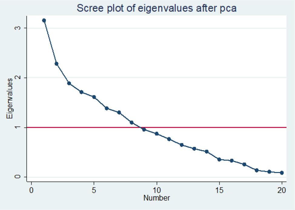
Scree plot of generated principal component
Source: own analysis.
As a result, these eight components were retained and rotated using varimax. On the other hand, sixteen variables with communalities greater than 0.4 were excluded from further analysis (Appendix 3). As a result, the logistic regression model used only four variables with communalities greater than 0.4 as regressors: acquisition of agrochemicals and fertilizers, increased use of hired labour, increased use of optimal input combination, and annual profit per acre. The Kaiser-Meyer-Olkin test sampling adequacy result of 0.621 is greater than the desired 0.500, indicating that the dataset is suitable for PCA analysis. The p-value for Bartlett’s test is statistically significant at the 5% level of significance (p-value = 0.000), indicating that the produced components were uncorrelated and thus demonstrating the validity of PCA.
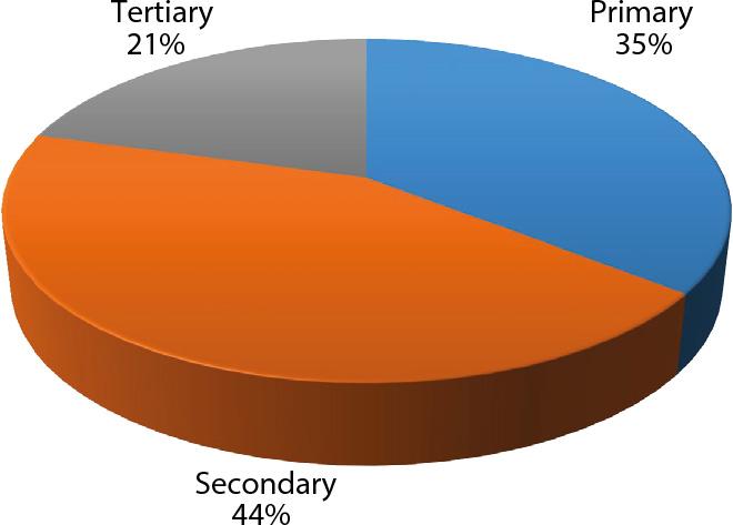
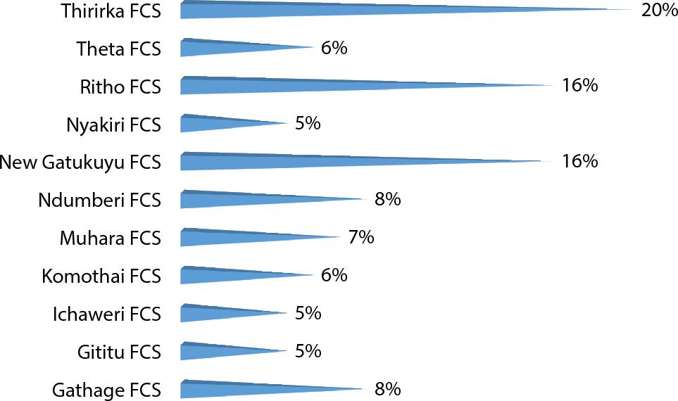
The summary statistics are shown in Figures 5 and 6, Table 5, and Appendix 4. Figure 5 shows that the majority (44%) of farmers who took part in the study had a secondary education. Farmers with tertiary education were the smallest group (21%), followed by those with a primary education (35%). Farmers who participated in the study came from eleven FCSs, as shown in Figure 6. Thiririka FCS accounted for the majority (20%) of farmers. Farmers at Ritho FCS and Gatukuyu FCS both accounted for 16%. Nyariki FCS, Ichaweri FCS, and Gatitu FCS each accounted for 5% of the farmers included in the study. Farmers at Theta FCS and Komothai FCS contributed 6% each. Ndumberi and Gathage FCS each contributed 8% of the farmers, and Muhara FCS contributed 7%.
The level of education of SHCFs (n = 174)
Source: own primary data.
The Percentage of SHCFs as per Affiliation of Farmers’ Cooperative Societies (n=174)
Source: own primary data.
How farmers used their agricultural credit
| Agricultural purpose | Frequency | Percentage (%) |
|---|---|---|
| Acquisition of new land | 7 | 25.0 |
| Land preparation (clearing, stumping among others) | 10 | 35.7 |
| Buying of inputs (fertilizers, agrochemicals, seedlings etc.) | 25 | 89.2 |
| Hiring of labour | 23 | 82.1 |
| Increase of acreage of cultivation | 14 | 50.0 |
Note: Multiple response and n = 28.
Source: Akinnagbe and Adonu, 2014.
Appendix 4 contains a table of perceptions of study variables for farmers with and without credit organized by four thematic areas. The first thematic area (the impact of agricultural credit on demand for coffee inputs) included six variables (see Table 3). Among these six variables, farmers perceived agricultural credit to have a significant impact only on the acquisition of agrochemicals and fertilizers, with 83% of all farmers, 87% of borrowers, and 74% of non-borrowers believing that this was the case. As a result, farmers’ emphasis on acquiring agricultural inputs cannot be overstated (McArthur and McCord, 2017). For example, Mukasa et al. (2017) discovered that 50% of credit approved was directed toward the purchase of agricultural inputs to boost agricultural productivity. Similarly, as shown in Table 4, Akinnagbe and Adonu (2014) conducted a survey to determine how farmers use agricultural credit and discovered that 89.2% of farmers used their credit to buy inputs. Thus, in the short run, credit is thought to improve farmers’ liquidity and thus increase their purchasing power, enabling them to obtain necessary inputs (seedlings, fertilizers, and agrochemicals, among other things) to increase productivity (Mukasa et al., 2017). This concept is consistent with RET, which holds that farmers are rational and risk-averse (Vriend, 1996). Thus, farmers buy inputs to increase productivity (Arrow, 1982).
On the other hand, 93% and 96% of all farmers believed that agricultural credit had no impact on land leasing or purchasing, respectively. Consistent with the perceptions of all farmers, 90% of borrowers and 95% of non-borrowers believed credit had no impact on land leasing. Similarly, 90% of borrowers and 94% of non-borrowers believed credit had no impact on land purchases. This is consistent with the findings of Akinnagbe and Adonu (2014), who discovered that only 7% of credit is used to purchase land. Furthermore, 63%, 67%, and 60% of all farmers believed that agricultural credit had no impact on accessing printed and electronic information, purchasing coffee seedlings, and acquiring manure, respectively. The disparity shown here in terms of perceptions of accessing both printed and electronic information, acquiring tree seedlings, and acquiring manure can be reconciled with the recognition that utility varies among farmers. This is consistent with SEUT, which states that people have utility functions and beliefs with associated probabilities of outcomes and thus make different decisions (Savage, 1954).
The second theme included five variables (see Table 3), with 74% of farmers believing that agricultural credit only affected hired labor. Similarly, 64% of borrowers and 84% of non-borrowers saw agricultural credit as having an impact on hired labor. This result is consistent with the summary statistics presented in Table 4, which show that 82.1% of farmers used credit to hire labor (Akinnagbe and Adonu 2014). In contrast, 75% and 52% of all farmers believed that agricultural credit did not affect the increased use of child and family labor, respectively. This finding demonstrates that labor remains a challenge in coffee productivity and other forms of agricultural productivity, regardless of family size. It has been observed that the majority of children and youth are enrolled in schools and tertiary institutions, respectively, and thus are not readily available to work on coffee or agricultural farms. Other studies found that child labor in agricultural production was not significant (Van Rooyen et al., 2012; Shimamura and Lastarria-Cornhiel, 2010). Furthermore, 78% and 96% of all farmers believed that agricultural credit did not affect the increased use of ox-plough and tractors, respectively.
Similarly, the third theme had five variables (see Table 3), and 84% of all farmers saw agricultural credit as having a significant impact on the increased use of the optimal combination of inputs. Similarly, 87% of borrowers and 82% of non-borrowers saw agricultural credit as having an impact on increased use of the best combination of inputs. According to prospect theory, which states that farmers view borrowed funds in terms of gains or losses (Kahneman and Tversky, 1979), farmers may be more inclined to farm coffee with inferior and low-return production technologies that require comparatively less working capital outlay rather than taking out loans to finance their coffee productivity and risking the loss of their properties. Nonetheless, 51%, 56%, 90%, and 64% of all farmers believed that agricultural credit did not affect the capacity to increase coffee farming areas, the acquisition of improved cultivars, increased access to extension services, or increased labor costs due to hired labor, respectively.
The fourth theme included four variables (see Table 3), with 78% and 54% of all farmers believing that agricultural credit increased annual profit per acre and wealth, respectively. Furthermore, 77% of borrowers and 78% of non-borrowers saw agricultural credit as increasing profit per acre. This demonstrates that the farmers were rational and bound by the RET axioms (EUT, SEUT, and PT). Thus, farmers would seek agricultural credit if they believed it would help them generate the highest expected returns while minimizing losses and risks. Nonetheless, farmer perceptions of return are consistent with those reported by Akinbode (2013), who linked agricultural credit to higher profits. Mukasa et al. (2017), on the other hand, argue that agricultural credit may help smallholder farmers create more wealth in the long run. Furthermore, 71% and 70% of all farmers believe that agricultural credit has no impact on the tendency to increase SACCO shares or invest in other businesses, respectively.
The two risk variables revealed that, on average, farmers were risk-averse. For example, 52% and 64% of all farmers said that obtaining agricultural credit could result in a loss and loan default, respectively. Similarly, 62% of borrowers and 90% of non-borrowers were concerned about loan default. When it came to the risk of losing money, 48% of borrowers were afraid of doing so. This proportion is lower than that of non-borrowers, with 56% unwilling to incur a loss as a result of securing agricultural credit. The proportion of non-borrowers and their perception of the danger of making a loss having acquired agricultural credit show risk rationing, which occurs when farmers refuse to obtain agricultural credit because they perceive it to be too risky (Binswager and Sillers, 1983; Boucher et al., 2008). The fear of 48% and 56% of borrowers and non-borrowers, respectively, about losing money can be explained with reference to prospect theory, which hypothesize that individuals are risk-averse with respect to gains and risk-acceptant with respect to losses and for its emphasis on the importance of the actor’s framing of decisions around a reference point (Kahneman and Tversky, 1979; Levy, 1992). Similarly, while coffee farming may be profitable at a certain capital-collateral mix, fear of default may prevent 62% of borrowers and 90% of non-borrowers from borrowing to avoid losing prime property pledged as collateral.
Table 6 summarizes the explanatory variables (acquisition of agrochemicals and fertilizers, increased use of hired labor, increased use of the optimal combination of inputs, and annual profit per acre) as well as the independent variable. Increased use of optimal input combinations had the highest mean of 0.844 but the lowest standard deviation of 0.363. In contrast, increased use of hired labor had the lowest mean (0.741) but the highest standard deviation (0.439). The acquisition of agrochemicals and fertilizers had mean and standard deviation values of 0.827 and 0.378, respectively. Annual profit per acre had a mean and standard deviation of 0.781 and 0.414, respectively. Nonetheless, all of the regressors are negatively skewed, indicating that the dataset is not normally distributed. This means that the tail on the left of the distribution is flatter than the tail on the right. The acquisition of agrochemicals and fertilizers (kurtosis = 4.008) and the increased use of optimal input combinations (kurtosis = 4.628) are leptokurtic (fat-tailed), with kurtosis greater than three. Finally, the increased use of hired labor (kurtosis = 2.215) and annual profit per acre (kurtosis = 2.858) are platykurtic (thin-tailed), with kurtosis less than three.
Summary statistics of regressors and regressand
| Variable | Mean | Standard deviation | Skewness | Kurtosis |
|---|---|---|---|---|
| Acquisition of agrochemicals and fertilizers | 0.827 | 0.378 | −1.734 | 4.008 |
| Increased use of hired labour | 0.741 | 0.439 | −1.102 | 2.215 |
| Increased use of optimal combination of inputs | 0.844 | 0.363 | −1.904 | 4.628 |
| Annual profit per acre | 0.781 | 0.414 | −1.363 | 2.858 |
| Influence of agricultural credit on coffee productivity | 0.787 | 0.410 | −1.404 | 2.972 |
Note: For all variables, minimum = 0; maximum = 1; and n = 174.
Source: results estimates.
The logistic regression results shown in Tables 7, 8, and 9 were fitted to the model Eqs. 2, 3 and 4, respectively. Table 7 shows the results for borrowers’ perceptions; Table 8 shows the results for non-borrowers’ perceptions; and Table 9 sums up the results for all farmers.
Perceptions of borrowers
| Regressor | Coefficient | Odds ratio | Standard error | p-value |
|---|---|---|---|---|
| Acquisition of agrochemicals and fertilizers | 2.470 | 11.821 | 1.063 | 0.020 |
| Increased use of hired labour | −2.146 | 0.116 | 1.035 | 0.038 |
| Increased use of optimal combination of inputs | −4.278 | 0.013 | 1.515 | 0.005 |
| Annual profit per acre | 4.128 | 62.075 | 1.100 | 0.000 |
| Constant | 1.729 | 5.636 | 1.119 | 0.122 |
Prob > χ2 = 0.0000; Pseudo χ2 = 0.3478; Log likelihood = −28.926159; n = 87; and LR χ2 (4) =30.86.
Source: results estimates.
Perceptions of non-borrowers
| Regressor | Coefficient | Odds ratio | Standard error | p-value |
|---|---|---|---|---|
| Acquisition of agrochemicals and fertilizers | 3.116 | 22.558 | 0.877 | 0.000 |
| Increased use of hired labour | −0.343 | 0.709 | 0.807 | 0.671 |
| Increased use of optimal combination of inputs | −1.706 | 0.181 | 0.998 | 0.088 |
| Annual profit per acre | −0.732 | 0.480 | 0.806 | 0.364 |
| Constant | 1.302 | 3.677 | 1.078 | 0.227 |
Prob > χ2 = 0.001; Pseudo χ2 = 0.196; Log likelihood = −36.709; n = 87; and LR χ2 (4) =17.91
Source: Results estimates.
Perceptions of all farmers (borrowers and non-borrowers)
| Regressor | Coefficient | Odds ratio | Standard error | p-value |
|---|---|---|---|---|
| Acquisition of agrochemicals and fertilizers | 2.040 | 7.691 | 0.811 | 0.012 |
| Increased use of hired labour | −1.111 | 0.329 | 0.580 | 0.056 |
| Increased use of optimal combination of inputs | −2.045 | 0.129 | 0.735 | 0.005 |
| Annual profit per acre | 3.262 | 26.114 | 0.612 | 0.000 |
| Constant | 1.447 | 4.251 | 0.717 | 0.044 |
Prob > χ2 = 0.0000; Pseudo χ2 = 0.223; Log likelihood = −69.938; n = 174; and LR χ2 (4) = 40.19.
Source: results estimates.
Tables 7, 8, and 9 provide the coefficients for logistic regression models 4, 5, and 6, respectively. The odds ratios in the respective tables can be used to interpret the logistic regression model results. For example, it can be deduced from Eq. 4 that farmers who acquired agricultural credit to produce coffee perceived that with an increase in agricultural credit of one Kenya shilling: (i) the likelihood of acquiring agrochemicals and fertilizers increases by a factor of 11.822; (ii) the likelihood of hiring labor decreases by a factor of 0.117; (iii) the likelihood of using the optimal combination of inputs decreases by a factor of 0.014; and (iv) the likelihood of increasing annual profit per acre of coffee increases by a factor of 62.076.
Secondly, it can be deduced from Eq. 5 that a farmer who didn’t secure agricultural credit to produce coffee perceived that with an increase in agricultural credit of one Kenya shilling: (i) the likelihood of acquiring agrochemicals and fertilizers increases by a factor of 22.558; (ii) the likelihood of hiring labor decreases by a factor of 0.709; (iii) the likelihood of using the optimal combination of inputs decreases by a factor of 0.182; (iv) the likelihood of increasing annual profit per acre of coffee increases by a factor of 0.481.
Finally, it can be deduced from Eq. 6 that borrowers and non-borrowers believed that with an increase in agricultural credit of one Kenya shilling: (i) the likelihood of acquiring agrochemicals and fertilizers increases by a factor of 7.691; (ii) the likelihood of hiring labor decreases by a factor of 0.328; (iii) the likelihood of using the optimal combination of inputs decreases by a factor of 0.129; and (iv) the odds of annual profit per acre or increasing annual profit per acre of coffee (versus non-increasing annual profit per acre of coffee) increase by a factor of 26.115.
Models 4, 5, and 6 affirm that both borrowers and non-borrowers perceive agricultural credit as having a positive impact on the acquisition of agrochemicals and fertilizers. Besides, the probability values for the acquisition of agrochemicals and fertilizers for borrowers (p value = 0.020), non-borrowers (p value = 0.000) and all farmers (p value = 0.012) are statistically significant. Similarly, Models 4 and 6 affirm that borrowers and all farmers perceive agricultural credit as having a positive impact on annual profit per acre of coffee. However, the non-borrowers alone perceive agricultural credit as having a negative impact on annual profit per acre of coffee. These results are consistent with those of Shah et al. (2008), who investigated the impact of credit on crop productivity and profit for farmers in the Chitral District in Northern Pakistan in 2007. Using descriptive statistics, their study found that credit had a positive impact on both inputs and profits. On the contrary, Nakano and Magezi (2020) assessed the impact of credit on the adoption of farm technology and productivity in Tanzania using a randomized control trial. Their results indicated that credit does not increase utilization of chemical fertilizer, productivity, profit from cultivated crops, or household income.
Models 4, 5 and 6 affirm that both borrowers and non-borrowers perceive agricultural credit as having a negative impact on hiring labor. This is because as you employ more labor in coffee production, each additional unit of labor contributes less to the overall output given that the marginal product of labor is diminishing, thus translating into less productivity per acre (Wicaksono, 2014). On the other hand, Seven and Tumen (2020) examined cross-country evidence of a relationship between agricultural credit and agricultural productivity using data for 24 consecutive years (1991 and 2014) for 104 emerging and developed countries. Using IV-2SLS regressions, the results indicate that a doubling of agricultural credit increases agricultural labor by about 4% more in emerging economies than in developing economies. However, most cross-country research assumes that all countries (in this case 104) boast a homogenous economic topology. Consequently, the “blanket-like” findings of cross-country studies don’t have serious policy ramifications for any given country.
Models 4, 5, and 6 affirm that both borrowers and non-borrowers perceive agricultural credit as having a negative impact on the use of the optimal combination of inputs. This result is inconsistent with Laha (2013) and Abdallah (2016), who found a positive relationship between agricultural credit and efficiency. For instance, Laha (2013) investigated the nexus between agricultural credit and efficiency in West Bengal in India using stochastic frontier analysis. The findings of this study indicated that farmers who received agricultural credit were much more efficient than farmers who did not receive credit. Laha (2013) indicated that the farmers with credit were more efficient because they directed the credit obtained to acquire the optimum combination of inputs. Similarly, Abdallah (2016) assessed how agricultural credit influences the technical efficiency of farmers of maize in Ghana using the Maximum Likelihood Method. The results of this study revealed that agricultural credit increased technical efficiency by 3.8%. However, unlike Laha (2013) and Abdallah (2016), this study focuses on the perceptions of farmers and does not deal with actual credit inputs and outputs.
The existing literature contains contradictory ideas about the effect of agricultural finance on agricultural production. This study investigated perceptions of the impact of agricultural financing on coffee productivity. It looked specifically at perceptions of the impact of agricultural loans on coffee input demand, hired labor, coffee production efficiency, and coffee production returns. According to the study’s findings, farmers perceive agricultural finance as having a positive impact on demand for coffee input and returns but a negative impact on demand for labor and coffee productivity efficiency. As a result, this study recommends that lenders restructure their lending policies to include all farmers, which would sustainably encourage economic change and significantly increase coffee productivity. The interactive model was not addressed in this study due to its complexity. As a result, for the provided empirical model, this study suggests using a factorial interaction model to combine farmer perception variables.