Crop diversification, as described by Ngure et al. (2020), is the redistribution of agricultural resources that include labor, land, capital, and farm implements towards the growing of more than one crop in a given year that has greater nutrition, is economically viable, or is more stress-resilient. According to some authors, crop diversification is considered one of the most effective agricultural development techniques that stabilizes household income (Kurdyś-Kujawska et al., 2021), alleviates poverty (Feliciano, 2018), decreases food insecurity (Mengistu et al., 2021, Douyon et al., 2022), and reduces production risks (Makate et al., 2023) and climatic risks (Makate et al., 2016; Awiti et al., 2022, and Vernooy, 2022). Anderzén et al. (2020) reported that smallholder coffee farmers adopted crop diversification strategies to reduce financial vulnerability, food insecurity, and the challenges of climate change.
Crop diversification insulates smallholder farmers from price volatility and market fluctuations, as well as reducing the likelihood of crop losses caused by pests, diseases, and adverse weather conditions (Beban and Gironde, 2023). Further, Mzyece and Ng'ombe (2020) reported that technical efficiency of 0.48 units and income variability of 0.007 units were reduced when there was a one-unit increase in the crop diversity index among rural farmers. In addition, Gezahegn et al. (2022) reported that intercropping haricot bean with cassava had a larger economic benefit of Ebirr 52219.8 with a land equivalent ratio (LER) of 1.54, since the legumes provided the cassava with additional yield during its early stages of growth.
In Kenya, the agricultural sector continues to be a key economic driver of development in Kenya's Vision 2030 and Sustainable Development Goals (SDGs), and with the current impacts of climate change and emerging pests and diseases posing challenges to agriculture production, agricultural policy recognizes the need for crop diversification to enhance food and nutrition security (GoK, 2021). However, there are no specific policies relating to food crop diversification, with the food crop diversification intensities among smallholder farmers remaining low and insufficient, thus hampering the country's effort towards sustainable rural development in many ways and reducing farmers' resilience (Awiti et al., 2022). In Kirinyaga East and Central Sub-Counties, smallholder farmers dominate the agriculture sector, and they face many productivity challenges such as socio-economic conditions, environmental factors, resource unavailability, low soil fertility, poor infrastructure, and the effects of climate change. To cope with income instability, food and nutrition insecurity, and marketing risks, crop diversification would be an effective strategy.
Different studies (including Makate et al., 2016; Derso et al., 2022; Maru et al., 2022; Gniza and Loa, 2023; and Makate et al., 2023) have shown that crop diversification can be shaped by various factors within farm households, such as socio-economic (household characteristics, land availability, farm size, income, market availability), institutional (group membership, credit, and extension service access), and also environmental factors (climatic and soil conditions) that affect farm diversification in various regions and countries. However, there has been limited research examining the determinants of crop diversification at the household level in the area studied here. As part of our contribution towards the achievement of sustainable development goals 1 and 2 on poverty reduction and enhanced food and nutrition security, respectively, in Kirinyaga East and Central Sub-Counties, this research was intended to examine and analyze the factors affecting the decision and extent of crop diversification by smallholder coffee farmers in the study area.
Theorization of crop diversification in the context of smallholder coffee farmers was guided by utility maximization theory. A household's decision to diversify was considered a major economic decision which had a strong bearing on the livelihoods of farmers. Utility maximization theory was used in this study because farmers base their decision to diversify crops on the agricultural household (Taylor and Adelman, 2003). Crop diversification is said to involve choices on production strategy that increase resilience and improves economic benefits. Using the Random Utility Model (RUM), the choice of smallholder farmer for crop diversification strategies can be envisioned using producer and consumer theory (Singh et al., 1986). This is due to the fact that it is excellent at modeling discrete choice decisions. Subject to uncertainty brought on by climate change, consumption costs and output prices, a farmer's production decisions, including optimal allocation, are thus dependent on their attitude towards risk and output produced, which maximizes farm household utility. Farmers in developing countries tend to be risk-averse and crop diversification may be a better strategy for them to insure against production risks (Hitayezu et al., 2016).
Uij represents the utility farmer i receives for participating in the jth crop diversification process, j assumes the value of 0 and 1 for no diversification and complete diversification, respectively. Thus, the utility derived from crop diversification by the ith farmer is subject to X, which is a vector of farm and farmer attributes of the diversifier and a vector of factors related to crop diversification. Therefore, the relation between the utility derivarable from the jth diversification process is hypothesized to be a function of the vector of observed farm, farmer and crop diversification specific characteristics with zero mean random error as expressed in Equation 1 and Equation 2.
Farmer i will choose to participate in crop diversification only if the utility derived from participating is greater than the utility from not participating. That is, a smallholder farmer adopts crop diversification if (Ui1 > Ui0). The only thing that can be observed is characteristics of household and attributes of the alternatives as faced by the decision-maker, since utilities are not observable. The following latent structure model for participation in crop diversification can express the utilities.
Z_i^*
The study was conducted in Kirinyaga East and Central Sub-Counties located in Kenya's Kirinyaga County, which is bordered to the north and east by Nyeri County, to the west by Murang'a County, and to the east and south by Embu County. It is located between Longitude 37°10′0″ E and 37°30′0″ E and latitudes 0°10′0″ S and 0°40′0″ S. The county, which has three agro-ecological zones (lowlands, midlands, and highlands) and is situated between 1,158 meters and 5,380 meters above sea level, is situated on the south-eastern slopes of Mount Kenya. There is a bimodal pattern in rainfall, with heavy rains (averages 2,146 mm) from March to May and short rains (averages 1,212 mm) from October to November. There is also variation in food production and consumption. During the hot season, the mean temperature varies from 18.4°C in the upper zones to 30.3°C in the lower zones. The majority of people live in rural areas, where agriculture is the main source of income (County Government of Kirinyaga, 2018).
Kirinyaga Central Sub-County and Kirinyaga East Sub-County hold significant importance in comprehending the consequences of crop diversification adopted by smallholder coffee farmers. They are characterized by high population density, a high coffee production level, favorable agricultural potential, several agro-ecological zones; the majority of farmers are small-scale, owning less than two hectares of land and also with high number of agricultural markets (Jaetzold et al., 2006). The kinds of crops planted are influenced by the various agro-ecological zones. The region is home to a variety of annual and perennial crops, including sweet potatoes (Ipomea batatas L.), vegetables, fruits, coffee (Coffee spp.), tea (Camellia sinensis L.), maize (Zea mays), beans (Phaseolus vulgaris L.), bananas (Musa spp.), and banana plants. These two sub-counties were chosen because of their capacity to produce a wide variety of food crops and their comparatively prominent involvement in agricultural and commercial operations (Fig. 1) (Jaetzold et al., 2006].
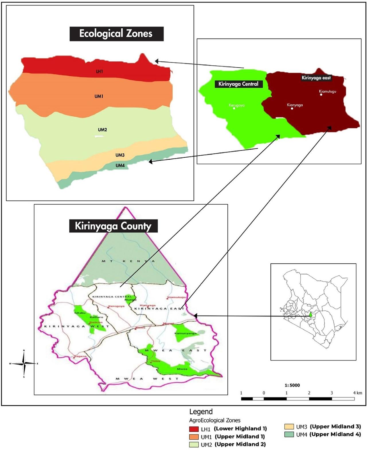
Thematic map of Kirinyaga Central Sub-County and Kirinyaga East Sub-County
Source: GeoCurrents (2015).
The study used descriptive survey design. It focused more on making specific predictions, narrating facts and features about people, groups or circumstances. This study design was appropriate, since it was of help in examining, characterizing and explaining the factors influencing smallholder coffee farmers on making decisions to diversify their crops and also to what extent.
The target population was 18420 smallholder coffee farmers in Kirinyaga Central (6777) and Kirinyaga East (11643) Sub-Counties (County Government of Kirinyaga, 2019), where ecological zones. The study employed the Cochran (2007) formula to calculate the sample size, which was estimated to be 408 households, and were chosen based on the population size of each strata selected in order to produce a sample for each agro-ecological zone. According to Minai et al. (2014), approximately 25% of the coffee farmers are in UM1, 50% in UM2 and about 25% in UM3.
p1 – represents the proportionate of population included in stratum 1, n – denotes the size of the entire sample and n·p1 – denotes the number of smallholder coffee farmers chosen from stratum 1, UM1 – is the coffee-tea zone, UM2 – is the main coffee zone and UM3 – is the marginal coffee zone. As a result, population size and sample size adopted a proportional allocation for each stratum in region of the study (Table 1). The study used a sample size of 408 smallholder farmers drawn from a population of 18420, which is divided into two Sub-Counties and three strata.
Sample size of smallholder coffee farmers in the study area
| Sub-County | AEZs | Location | Sub-Location | Population | Sample Size |
|---|---|---|---|---|---|
| Kirinyaga Central | UM1 | Mutira | Kabari | 911 | 20 |
| Inoi | Mbeti | 500 | 11 | ||
| UM2 | Kerugoya | Kaitheri | 1 900 | 42 | |
| Koroma | Nduini | 922 | 20 | ||
| UM3 | Kanyekini | Kianjege | 2 174 | 48 | |
| Kutus | Kangu | 370 | 08 | ||
| Kirinyaga East | UM1 | Ngariama | Rungeto | 600 | 13 |
| Karumandi | Kiaruri | 2 222 | 50 | ||
| UM2 | Baragwi | Rwambiti | 3 200 | 71 | |
| Njukiini | Ngiriambu | 2 800 | 62 | ||
| UM3 | Kirima | Mutige | 1 490 | 33 | |
| Kabare | Rukenya | 1 331 | 30 | ||
| Totals | 18 420 | 408 | |||
UM1 – Upper midland 1, UM2 – Upper midland 2, UM3 – Upper midland 3 and AEZs – agro-ecological zones.
Source: County Government of Kirinyaga, 2019.
A multistage sampling technique was used, where in the first stage, Kirinyaga central and Kirinyaga East Sub-Counties were purposively selected due to their prominence as significant coffee-growing regions in Kirinyaga County. In the second stage, three agro-ecological zones suitable for coffee production were chosen through stratification, and they included the coffee - tea zone (Upper Midland one – ), the main coffee zone (Upper Midland two – ), and the marginal coffee zone (Upper Midland three –. In the third stage, 12 sub-locations were randomly chosen from each of the 12 locations in the three AEZs. Next, smallholder coffee farmers were randomly selected from the 12 sub-locations. Finally, the sample size needed for each stratum was used to determine how many smallholder coffee farmer households were chosen.
Before actual data collection, a pilot study was conducted in Runyenjes Sub-County, Embu County, where 38 questionnaires (10% of the sample size) were pre-tested before the actual survey among smallholder coffee producers. Face-, content- and construct validity were examined, and piloted data was also used to assess the instrument's reliability through use of the Cronbach's coefficient alpha. The questionnaire items were found to have a reliability value of 0.820, which is above 0.7 (acceptable level). Data from smallholder coffee producers were gathered using structured questionnaires administered on Android phones and tablets using the free open-source program Kobo Toolbox (https://www.kobotoolbox.org/). The structured questionnaire was used to capture socio-economic and demographic information of smallholder coffee farmers, which was used to capture individual-level heterogeneity such as gender, age, education level, extension services, land size, distance to market, cooperative membership and credit access. The survey took between 30 and 50 minutes to complete. The survey obtained information on the factors influencing farmers to diversify and extent of diversification.
In this study, STATA version 15 was employed to analyze data where descriptive statistics such as mean, standard deviations, percentages and frequencies were used to address the first objective, which profiled the socio-economics characteristics of smallholder coffee farmers. Inferential statistics were obtained from Cragg's double-hurdle model to examine the determinants of household decisions and the extent of crop diversification among smallholder coffee farmers in Kirinyaga Central and Kirinyaga East Sub-Counties.
The study sought to identify factors determining coffee producers' participation decisions and level of crop diversification. In addition, this study explored the factors that significantly influenced participation decisions and how they related to the dependent variables. As a result, the following dependent and independent variables were established and postulated in this investigation. (Table 2).
Summary of the explanatory variables used in the double-hurdle model
| Variable | Description | Exp sign |
|---|---|---|
| Explained variables | ||
| Crop diversification choice | Binary: 1 if the farmer uses at least 1 crop diversification strategy, 0 if otherwise | |
| Crop diversification extent | Crop Diversification Index (0–1) | |
| Explanatory variables | ||
| Gender of the household head | Binary: 1 if the gender of the farmer is male, 0 if otherwise | +/− |
| Age of the household head | Continuous: Age of household head (Years) | +/− |
| Education level of the household head | Continuous: Highest level of education attained | + |
| Extension access | Binary: 1 if the farmer had accessed extension services, 0 if otherwise | + |
| Group membership | Binary: 1 if the farmer was a member of a community organization, 0 if otherwise | + |
| Household size | Continuous: Number of dependents in the household | + |
| Distance to market | Continuous: Walking distance to market in km | +/− |
| Access to credit | Binary: 1 if the farmer had received inputs credit, 0 if otherwise | + |
| Total cultivated land size | Continuous: The total cultivated land size (Ha) | +/− |
−/+indicates listed variables were expected to affect crop diversification negatively or positively.
Source: author's conceptualization, 2022.
The Herfindahl Index (HI) was employed to measure crop diversification, since it is one of the most generally employed indexes in the crop diversification literature (Asante et al., 2017; Mengistu et al., 2021 and Appiah-Twumasi and Asale, 2022). It is a measure of how evenly a farmer spreads their land and resources across different crops. The crop diversification index (CDI) is a concentration index. As a result, CDI was used to assess crop diversification. The formula devised by Hirschman (1964) in Equations 5 and 6 was used to compute HI, which is the sum of squares of all n proportions:
Pi = proportion of ith crop, Ai = Area under ith crop (ha), Σni=1Ai is the total cropped land (ha), and 1 is the number of crop i.e. 1, 2, 3, …, n
Subtracting the HI from 1 and 0 yielded the CDI values (equation 7). Furthermore, a crop diversification index value of 0 implies perfect specialization, while a trend towards 1 indicates a rise in the extent of agricultural diversification (Gniza and Loa, 2023).
In general, the CDI value rises when diversification increases and falls to zero when producers plant and nurture a sole crop. The producers in this research study mostly grow maize, beans, cabbage, kale, bananas, avocado, cowpeas, sweet potatoes, potatoes, tomatoes, French beans, arrow roots, cassava, and pumpkin. To calculate the Herfindahl index, total cropped land (ha) for the diversifiers and the ratio of land allotted for producing each crop per ha in the harvest season of 2021/2022 were used.
To determine the choice and level of crop diversification, Cragg's double-hurdle model was employed for this study because two decisions were taken at several stages, and similar factors had varying effects on the two decisions (Asfaw et al., 2022). According to Tura et al. (2016), the Heckman, Tobit and double-hurdle models are the most common approaches for modeling the choice and extent of crop diversification circumstances. The double-hurdle procedure is a more flexible parametric generalization of the Tobit and Heckman models that enables two distinct stochastic processes to influence one's choice to participate and the crop diversification level. The 1st stage (probit) and the 2nd stage (truncated regression) models must be applied jointly, either sequentially or concurrently to provide asymptotically efficient and consistent estimates for all of its parameters (Derso et al., 2022). Following Gniza and Lao (2023), the theoretical foundation for the Cragg's (1971) double-hurdle estimating framework is the probit model, in which the likelihood of crop diversification at observation t, denoted by P(Et), is given by:
Xt – is a vector K x 1 of variables exogenous to observation t and β represents a vector of parameter estimates. C(z) is the cumulative unit normal distribution as shown in Equation 9.
The first stage of the probit model is used to estimate the probability of a producer to diversify crops or not. The second stage determines how much diversification should be applied to land acreage. Only non-zero values in the first stage can be employed to estimate the level of crop diversification in stage two by use of the truncated regression model. The model presupposes that at least one explanatory variable from the first equation must be absent from the second stage of identification because it expects the inclusion of one or more variables in the selection rather than the output equation. This means that the choice and extent of crop diversification were not determined by a closely related set of explained variables. In this study, group membership was the only identifier variable that influenced just the first stage (probability of diversification) but not the second stage (extent of diversification) of the selected diversification strategies. A double-hurdle model was therefore adopted for this study, which is specified in Equation 10 as:
CDi* is latent variable that denotes binary censoring or the choice in our study
Taking value of 1 for diversity of crops and 0 suggests the opposite. QCD** is the latent variable that represents the number of diverse crops.
The second decision on the extent of diversification of crop is elaborated in Equation 12 as:
The double-hurdle log-likelihood function, which nests the probit model and truncated regression is denoted as:
Φ is the standard normal probability function and ∅ as the density function. Zi and Xi represent probit and truncated model explanatory variables respectively. α, σ, and β were parameters to be predicted for each model.
The findings indicates that households head in the study area had an average age of 48.6 years, with a standard deviation of 13.31 (Table 3). This shows that the vast majority of the survey participants were within the active labor force, had extensive farming experience and were risk-averse. It is probable that older farmers have greater access to production resources and information may impact their decision to diversify. This is in line with the findings of Dembele et al. (2018), who stated that producers in Mali are likely to adopt crop diversification as they age. Regarding the education level, household heads had completed 10.8 years in school, which was the minimum required educational level (Table 3). This may have implied that farmers were more likely to have more knowledge and skills, resources and also be better informed about agricultural instructions and information provided by extension officers. This would help them to identify new crops that are in demand and adapt more diverse farming practices accordingly. Mulwa and Visser (2020) reported that highly educated heads of household diversify crop farming more compared to their counterparts, as farmers with a higher education level may be more likely to engage in research and experimentation, which would allow them to explore and adopt new crop varieties and farming methods.
Demographic characteristics of discrete variables
| Variables | Mean | Std. Dev |
|---|---|---|
| Age (years) | 48.01 | 11.43 |
| Education level (years) | 10.82 | 3.19 |
| Household size (No.) | 3.63 | 1.05 |
| Distance (km) | 2.36 | 0.09 |
| Land size (ha) | 1.59 | 0.41 |
| Cropped land (ha) | 0.58 | 0.13 |
Source: field survey, 2022.
The study further revealed that the average membership size of a household was 4 persons, which reflects the human capital availability for agronomic activities (Table 3). It is possible that a larger household may provide more hands to help with farming activities, which can make it easier to manage a diverse range of crops. Appiah-Twumasi and Asale (2022) noted that larger household sizes have more individuals available to contribute to agricultural activities, which allows for the cultivation and management of multiple crops. The average distance between the sampled households and the closest marketplace was 2.4 km, with a range of 0.5 km to 8 km (Table 3). These findings may imply that the majority of the farmers were near the market area, and access to markets may boost farmers' incentives to diversify crops and grow surplus food crop that can be conveniently carried to market, thereby increasing their income. This study's findings are consistent with those of Maru et al. (2022), who noted that proximity to markets provides a way of exchanging and sharing information among small-scale producers and providers of services; thus, producers closer to marketplaces are highly inclined to diversify crops.
The findings showed that the average land size (1.59 ha) of the respondents was less than 2 hectares (Table 3). It is possible that smaller land sizes limit ability to diversify, but through implementation of crop diversification strategies like intercropping, farmers can obtain more yields. Lv et al. (2023) noted that farmers need to implement measures such as crop rotation and intercropping to boost soil fertility, which may result in increased crop yields regardless of land size. Further, during this study it was observed that the mean total cropped land was 0.91 ha per household, which meant that more than half of the total land area was used for growing a variety of food crops (Table 3).
About 68.83% of the households surveyed were headed by men, whereas the remaining 31.17% were headed by women (Table 4). This could imply that most of the households in the area studied are male-dominated and can cultivate various crops on a particular plot of land because men can access factors of production more easily than females. During the study, it was found that 37.5% of the respondents had diversified their crops in less than 10 years (Table 4), which implies that farmers in the research area had less experience in crop diversification, probably due to low years of carrying out the practices. Makate et al. (2023) noted that farmers who had acquired experience from earlier crop diversification had a better probability of intensifying subsequent diversified systems and of adapting to recurring rainfall shocks.
Demographic characteristics of categorical variables
| Variables | Category | Frequency | Percent. |
|---|---|---|---|
| Household head | Female | 125 | 31.17 |
| Male | 276 | 68.83 | |
| Diversification (years) | Less than 10 years | 150 | 37.4 |
| 10–20 years | 115 | 28.68 | |
| Above 20 years | 136 | 33.92 | |
| Extension (access) | No | 112 | 27.93 |
| Yes | 289 | 72.07 | |
| Extension often | Once | 17 | 5.88 |
| Twice | 53 | 18.34 | |
| Thrice | 85 | 29.41 | |
| More than thrice | 134 | 46 | |
| Group membership | No | 20 | 4.99 |
| Yes | 381 | 95.01 | |
| Group benefits | Agricultural information | 180 | 47.24 |
| Marketing information | 39 | 10.24 | |
| Credit access | 96 | 25.2 | |
| Input access | 66 | 17.32 | |
| Credit access | No | 51 | 12.72 |
| Yes | 350 | 87.28 | |
| Diversifiers | No | 21 | 5.24 |
| Yes | 380 | 94.76 |
Source: field survey, 2022.
This study's findings showed that 72.07% of the heads of households accessed services provided by extension workers, where the majority of them accessed them more than thrice at 46% (Table 4). This may imply that farmers were capacitated through training by extension officers in good agronomic practices, marketing and business-oriented farming. Shangshon et al. (2023) noted that agricultural training in Bhutan helped farmers adopt production-enhancing technology and implement effective marketing techniques, such as the use of better varieties of crops, intercropping, optimum plant spacing, optimal fertilizer use and collective marketing.
The findings of this study showed that social groupings were a common component of social ties in rural agricultural households in Kirinyaga County, where 95.01% of the respondents were members of them. The findings revealed that 47.24% of the respondents joined producer groups to obtain agricultural information (Table 4). These findings may indicate that farmer groups are an important catalyst for adopting innovation and upgrading farming systems as recommended by extension officers and trainers through efficient information flows. In agreement with the study's observations, Kehinde et al. (2022) revealed that membership of an agricultural organization increased the intensity of soil conservation practices such as mulching among small-scale farmers in Nigeria.
The study finding showed that marketing information was a benefit to the social group at 10.24% (Table 4). This indicated that farmers could access marketing information through other channels such as extension visits, radios and social media. In Uganda, Hill et al. (2021) noted that market information is the main factor inducing market participation, since households know what is demanded, when to make a sale, to whom to sell to, and the right price. It is possible that through marketing information farmers are able to increase their market access due to economies of scale in procuring inputs, bargaining power in making sales and marketing produce collectively.
According to the findings of this study, the majority of the households studied accessed credit (87.28%), while 12.72% did not. These findings may imply that financial literacy is high and farmers access credit for agricultural activities. Olutumise (2023) reported that increased access to credit may incline farmers to devote resources to more expensive but more rewarding production practices in order to enhance smallholder farmers' livelihoods. According to the findings of this survey, more than three-quarters (94.76%) of farmers were crop diversifiers, while the remaining households (5.24%) were non-diversifiers (Table 4). This indicated that the majority of farmers were diversifying their crops to lower the chance of yield loss and boost farm resilience to pests, diseases and adverse weather conditions, while more resources, such as labor and equipment, were necessary to manage the strategy.
The findings of this study indicated that the mean crop diversification index in the study area was 0.39, while 65.09% of the diversified farmers had a CDI that oscillated between 0.1 to 0.4 and 29.92% had a CDI range of 0.5 to 0.8 (Table 5; Fig. 2). This implies that there was a low degree of diversification among small-scale farmers. These findings are comparable to those of Kanyua et al. (2013) and Awiti et al. (2022), who found a CDI of 0.34 and 0.42 in Gatanga (Murang'a County) and Kisumu West Sub-County, respectively. The study's findings are in line with those of Kanyua et al. (2013), who postulated that more than three-quarters (70.08%) of respondents showed an index of 0.4 and below.
Crop diversification level of sampled households
| Crop Diversification Index | Frequency | Percent. |
|---|---|---|
| 0–0.1 | 20 | 4.99 |
| 0.10–0.2 | 98 | 24.44 |
| 0.30–0.4 | 163 | 40.65 |
| 0.50–0.6 | 108 | 26.93 |
| 0.70–0.8 | 12 | 2.99 |
Source: field survey, 2022.
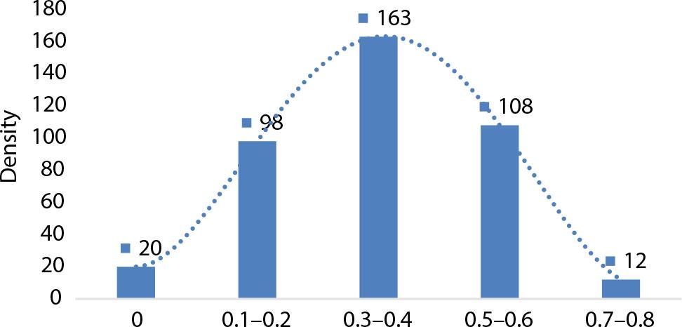
Crop diversification distribution in the study area
Source: field survey, 2022.
Based on the findings of this study, the crop diversification index household differentiation on small farms was influenced by farm and farmer characteristics, natural conditions, and area allocated to a crop. The findings indicated that households with low crop diversity were distinguished by small land holdings and a scarcity of labor as a result of small household sizes.
During the study period, it is possible that these households had low employment in agriculture and were also distinguished by a low level of adoption of crop diversification strategies such as intercropping, crop rotation, landscape heterogeneity, and crop species and varietal diversity. Kiryluk-Dryjska and Więckowska (2020) found that regions that had developed agricultural structures diversified more compared to areas with structural disadvantages, where diversification was needed more. Further, Kurdyś-Kujawska et al. (2021) noted that in Poland, regions with high crop diversity were characterized by low land and labor productivity caused by a predominance of poor soil fertility and agricultural culture. It was possible that greater diversity in crops was a rational behavior for smallholder farmers because they had to adapt to the improved crop diversification strategies to boost their crop diversity systems for food security and increased productivity.
A test for normality of CDI was conducted using kernel density plot residuals, which gave a reasonably and clean curve that closely resembled a normally distributed curve, showing that the assumption of normality was not violated (Fig. 3).
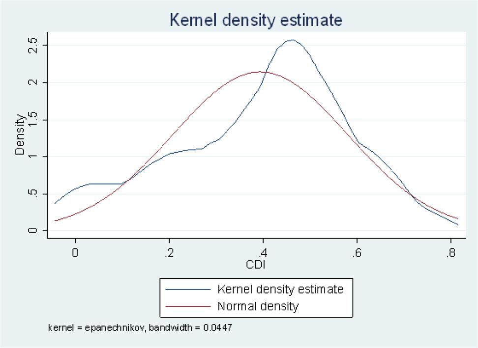
Kernel density estimate for crop diversification index
Source: field survey, 2022.
The kernel density estimate was able to select households with low and high diversification levels in the sample farms as a function of multiple characteristics and would be used as a dependent variable. The findings of this study are consistent with those of Nkonde et al. (2021), who found out that the kernel density plot in Zambia was less peaked and not skewed, which may have implied that the mean CDI would be used as the cutoff point to create a binary variable of whether a household diversified.
The findings of the decision model showed that the model was statistically significant at p < 0.05 with Wald chi-square (8) = 80.46, Pseudo = 0.618. The Wald chi test at p < 0.01 showed that independent variables jointly explain farmers' decisions to undertake crop diversification (Table 6). Thus, these findings showed that the model was a good fit. In turn this means that the value for this analysis was 0.618, suggesting that this model explains 61.8% of the variation in the dependent variable.
Probit regression estimates for determinants of crop diversifications
| Variables | Coeff. | Std. Err | z | p-value | dy/dx |
|---|---|---|---|---|---|
| Gender of household head | −0.466 | 0.306 | −1.520 | 0.129 | −0.062 |
| Age of household head (years) | −0.006 | 0.011 | −0.550 | 0.581 | 0.001 |
| Household size (No.) | 0.143* | 0.087 | 1.980 | 0.099 | 0.016 |
| Access to Extension services | 0.704** | 0.261 | 2.700 | 0.007 | 0.065 |
| Cooperative membership | 0.563 | 0.487 | 1.160 | 0.247 | 0.013 |
| Distance to the market (km) | −0.102 | 0.069 | −1.470 | 0.141 | −0.003 |
| Credit access | −0.618 | 0.550 | −1.120 | 0.262 | 0.027 |
| Land size (ha) | 1.058** | 0.322 | 3.290 | 0.001 | 0.088 |
| Education level (years) | −0.008 | 0.041 | −0.200 | 0.838 | 0.0047 |
| _cons | −0.227*** | 0.008 | 28.375 | 0.000 | |
| lnsigma | |||||
| _cons | −1.833 | 0.040 | −46.130 | 0.000 | |
| /sigma | 0.160 | 0.006 | |||
| LR chi2(8) | 80.46 | Pseudo | 0.618 | ||
| Prob > chi2 ( ) | 0.000 | Log likelihood | 105.327 | ||
| No. Observation | 401 | ||||
*, ** and *** represent statistical significance of factors at 10%, 5% and 1% levels, respectively.
Source: field survey, 2022.
The household size coefficient was positive and significant at the 10% probability level, showing a positive relationship between household size and decision to diversify. The finding presented by this study revealed that an increase of one person in the household leads to positive change in the probability of diversifying crops by 1.60% (Table 6). This may imply that with more land available, families may be able to grow a wider variety of crops, including those that require more space or specialized growing conditions. The findings of this study concurs with those of Gniza and Loa (2023), who found out that having more members in a household represents the potential availability of labor for producers, who are then more likely to engage in crop diversification. It is possible that large families are able to engage in multiple cropping systems compared to smaller families due to high labor availability and food security concerns. Conversely, Asante et al. (2017) reported a negative effect of the dependency ratio on discrete decisions, which may imply that with more family labor and a higher number of dependents, the probability of diversifying crops is smaller.
The findings of this study showed a positive and significant association between access to extension services per year and crop diversification with coefficient being significant at 5%. It is possible that the extension system resulted in the spread and adoption of innovation through the provision of technical advice, credit availability, market information provision, input supplies and capacity building of farmers. In relation to the findings of this study, an increase in access to extension services by one contact increased the probability of crop diversification by 6.5% (Table 6), which may imply that farmers were motivated to grow different crops to safeguard themselves against production and marketing risks. Similarly, Derso et al. (2022) found that extension contacts positively and significantly influenced crop diversification. Based on the findings of this study, accessibility of extension services focuses on enhancing farmers' productivity and increase income due to a reliable source of technical advice on current knowledge, better germplasm, other management aspects and market information.
The findings of this study revealed that land size positively and significantly affect probability of crop diversification at the 5% level of significance, whereas when the size of land holding increased by one hectare, the probability of the farmer to participate in crop diversification increased by 8.8% (Table 6). The positive impact of land size may imply that producers with relatively larger farms practice crop diversification more than smaller farms. The findings of this study concur with those of Dessie et al. (2019), who reported a positive relationship between land size and decision to diversify crops. This may imply that an increase in the availability of farmland may lead farmers to practice crop diversification. Similarly, Makate et al. (2016) found that in Zimbabwe a 1-acre increase in land size accessed by household increased the probability of adopting crop diversification by 15.8%.
In addition, Mandere et al. (2011) reported that Kenyan farmers who had a larger share of land had high probability of allocating their land area to a new crop, such as sugar beet, which reduced the land area of their plants currently in farm. In contrast, Derso et al. (2022) found that land size had a detrimental impact on the likelihood of diversification, which could imply that farmers may not be able to cultivate different crops due to the increased management skills and inputs required for huge acreage. Also, contrary to the findings of this study, Adjimoti et al. (2017) found out that larger land holdings in Benin were related to reduced diversity, owing to the fact that holders of large farm sizes tended to undertake diversification into high-value crops and subsequently specialized on cashew cultivation. From the findings of this study, it is possible that large farm landholdings may allow households to allocate their farms to the production of different types of crops than their counterparts with smaller farms.
The second stage of Cragg's double-hurdle model involved the use of truncated regression, which ensured that the coefficient estimates were interpreted in terms of the likelihood between the dependent variable (extent of diversification) and the independent variables. Thus, it was not necessary to generate marginal effects as in the first stage of the model. The key factors affecting the level of crop diversification include gender of household head, access to extension services, land size, education level, and household size (Table 7).
Truncated regression estimates for determinants of extent of crop diversification
| Variables | Coeff. | Std. Err | z | p-value |
|---|---|---|---|---|
| Gender of household head (Yes=1, No=0) | −0.053** | 0.018 | −2.960 | 0.003 |
| Age of household head (Years) | 0.011 | 0.01 | 1.100 | 0.241 |
| Access to extension services (Yes=1, No=0) | 0.052* | 0.020 | 2.540 | 0.011 |
| Distance to market (km) | 0.002 | 0.005 | 0.540 | 0.633 |
| Credit access (Yes=1, No) | 0.044 | 0.027 | 1.630 | 0.102 |
| Land size (ha) | 0.067** | 0.023 | 2.910 | 0.004 |
| Education level (years) | 0.005* | 0.002 | 1.980 | 0.048 |
| Household size (number) | 0.013* | 0.005 | 2.370 | 0.018 |
| Constant | 0.106*** | 0.027 | 3.926 | 0.000 |
| LR chi2(8) | 80.46 | Pseudo | 0.618 | |
| Prob > chi2 ( ) | 0.000 | Log likelihood | 105.327 | |
| No. Observation | 401 |
p < 0.001
p < 0.05
p < 0.1
Source: field survey, 2022.
During the study period, it was observed that gender of the household head negatively and significantly affected the extent of crop diversification at the 5% significance level, with male-headed households decreasing crop diversification level by 6.1% (Table 7). These findings may imply that women who were in charge of food preparation were more risk-averse than males, and were more concerned with providing diversified nutrition for the family and cultivating crops that are nutritious, such as legumes or vegetables, which motivated them to diversify crops more. The observations of this study are consistent with those of Assefa et al. (2022), who reported that female-headed households grew more diverse crop types, since the majority of them contributed labor for most farming operations, whereas male-headed households only made managerial decisions and sought other job opportunities to support their family livelihood system. On the other hand, Nidumolu et al. (2022) noted that women had limited independent decision-making authority due to minor positions being allotted to them in the traditional agricultural system, while men were more inclined to diversify due to their access to production resources, and better access to both information and technologies that would influence their decision-making with regard to the cropping system.
The findings of this study show that access to extension services was positive and significant at the 10% level, which would imply that farmers who had an increased number of extension contacts throughout cropping period improved the extent of crop diversity by 5.2% (Table 7). The study's findings revealed that extension access may expose producers to agricultural and marketing information, which may decrease the household's uncertainty associated with crop production and thus increase the level of crop diversification. In agreement to the outcomes of this study, Aheibam et al. (2017) reported that households with access to farming information in Manipur increased their level of crop diversification by 15%, which could imply that farmers who have a higher crop diversity extent resonated with extension advice and market information to this effect. Similarly, Mwololo et al. (2019) noted that in Kenya access to government and private extension services boosted total farm diversity by 84.9% and 90.7%, respectively, which could imply that farmers who used government and private extension services had more diverse farms.
The findings of this study showed that land size had a positive and significant effect (p < 0.05) on the level of crop diversification, where an increase in land by one hectare of resulted in change of crop diversification extent by 6.7% (Table 7). The findings of this study show that it is possible for farmers to maximize income and minimize production and price risks with larger farm size, since they would allot their land to multiple crops compared to small land holders. The findings of this study are consistent with those of Li et al. (2021), who found that larger farm sizes allow households to allocate more area to crops than small holdings because of the higher availability of cultivable land, which leads to greater crop variety. Further, it was noted that farmers with extensive landholdings would grow more crops to suit their nutritional needs or sell surplus harvests to boost their income. Moreover, Awiti et al. (2022) noted that larger land size enables farmers to use more advanced farming techniques and equipment, which can lead to increased efficiency and yields. On the other hand, Rehima et al. (2013) found an inverse relationship between farm size and the level of crop diversification, where they argued that having larger farmland beyond a certain limit required more management skills, inputs and technologies.
The findings of this study showed that education level had a positive and significant effect at 10% on the extent of crop diversification, where an increase by one year of education increased the extent of crop diversification by 0.5% (Table 7). These findings reveal that it is possible for farmers with higher education levels to increase their access and use of agricultural technologies and practices such as cropping systems and landscape heterogeneity, which enabled them to enhance their yields and improve their livelihoods. The findings of this study are consistent with those of Lawin and Tamini (2019), who found that farmers with more years of schooling had a higher extent of crop diversification, due to improved managerial capacity through education and training. The findings of this study are in agreement with those of Aheibam et al. (2017), who reported that a one-year increase in the formal education of the household head increased the level of crop diversification by 5%, which may imply that farmers were able to make constructive decisions to accept new ideas of adopting new crops varieties that produce more yields and are resistant to pest and disease, and also to use improved growing methods, which in turn lead to a wider range of crops being grown. Based on the findings of this study, higher education levels enable farmers to explore and adopt new crop varieties and species, thus resulting in a more diverse cropping system.
The findings of this study revealed that the coefficient on the number of people in the household was positive and significant at the 10% level, which implied a positive relationship between household size and the level of diversification, which may suggest that each additional member in a household increased the degree of crop diversification by 1.3% (Table 7). The findings of the study showed that it is possible for larger households to have greater labor resources, which would influence them in diversifying more compared to smaller-sized households. The findings of this study are consistent with those of Maru et al. (2022), who suggested that a larger family size provides labor to carry out multiple procedures on farms, such as land preparation, planting crops, sowing and harvesting, which in turn influenced the household head to add more varieties of crops. Contrarily, Alhassan et al. (2020) reported that large labor force would be costly to feed, mostly in the lean season, because larger households may have higher consumption needs, which may limit their ability to invest in agricultural inputs or increase diversification of crops.
Crop diversification is a critical issue for enhancing farmers' livelihoods in developing countries like Kenya. This study sought to examine the determinants and extent of crop diversification in Kirinyaga East and Kirinyaga Central Sub-Counties, Kirinyaga County. The study was motivated by the need to understand the socio-economic and institutional factors that influence farmers to diversify and also increase the extent of crop diversification, as the mean CDI in the study area was found to be low at 0.390. According to the study findings, household size, access to extension services, and land size were found to be the main factors that significantly influenced farmers' decisions to diversify their crops. The extent of crop diversification was mainly influenced by the gender of the household head, education level, household size, access to extension services, and land size.
Female-headed households were more involved in crop diversification compared to their male counterparts. Education and extension services are likely to increase the ability of the farmer to make better decisions to diversify crops, since they are able to understand agricultural information, adopt new innovations, and enhance their managerial capacity. The availability of more resources, such as land, provides greater opportunities for diversification, and new crops can be grown by experimenting with new pest control technologies or adopting sustainable land management practices. The information provided is key to providing favorable conditions and suitable environments for the acceptance and spread of crop diversification among smallholder farmers. This study recommends that extension officers should organize more workshops and seminars to educate smallholder farmers about the benefits of crop diversification and the economic advantages of growing a variety of crops. Also, offering hands-on training on crop diversification techniques like crop rotation and intercropping is advisable. There is also a need for the government to invest in and align formal education with agricultural training systems. This is a key practice for exploring and adopting new crop varieties and species, and leads to a more diverse cropping system.