
Publisher’s Note: A correction article relating to this paper has been published and can be found at https://b.tellusjournals.se/articles/10.16993/tellusb.1890.
1. Introduction
The abundance of aerosol particles that act as cloud condensation nuclei (CCN) can affect the radiative properties of clouds by altering the cloud droplet number concentration (Nd), the liquid water path (LWP) as well as the depth and lifetime of the clouds (Albrecht, 1989; Twomey, 1959; Twomey, 1974). Although significant progress has been made in understanding and quantifying aerosol-cloud interactions, substantial uncertainties remain in current global climate modeling estimates (Bellouin et al., 2020; Masson-Delmotte et al., 2021; Quaas et al., 2020). High-resolution models with sophisticated cloud microphysics (see, e.g., overview by Khain et al., 2015), i.e., large-eddy simulation (LES) or cloud-resolving models, are promising tools to further develop our understanding of aerosol-cloud interactions and help to improve the predictive power of large-scale models (Grabowski et al., 2018). Since the first exploitation of LES by Deardorff (1970), this modeling technique has greatly enhanced the scientific understanding of turbulent flows of atmospheric planetary boundary layers (e.g., Moeng and Sullivan, 2015; Stoll et al., 2020). Today, LES with cloud microphysical modules allows us to study complex cloud regimes with high detail, and the simulations are often used as a benchmark for models that cannot explicitly resolve the cloud scale. For example, LES has been suggested as a fundamental tool to investigate phenomena such as marine cloud brightening, i.e., the injection of aerosol particles in low-level marine stratocumulus clouds to increase their reflectivity and dampen global warming (Feingold et al., 2024). Therefore, it is also necessary to critically evaluate if these high-resolution models can skillfully simulate expected physical phenomena.
In this study, we focus on evaluating the skill of an LES model equipped with a bulk microphysical scheme to simulate the first indirect effect—also known as the Twomey or cloud-albedo effect—in a warm stratocumulus-topped boundary layer. Twomey (1974) first proclaimed that an increase in aerosol number (Na) will lead to smaller and more numerous Nd, which increases cloud albedo (under constant LWP). However, the susceptibility, , does not depend only on Na. An aerosol activates into a cloud droplet when the supersaturation in an air parcel exceeds the size-dependent equilibrium saturation ratio of the solution droplet (Köhler, 1921). In the atmosphere, supersaturation is most effectively created by adiabatic lifting, which leads to thermal expansion and cooling and, hence, an increase in relative humidity (RH) as the saturation vapor pressure decreases. As RH increases, particles (e.g., soluble aerosols or droplets) take up water by condensational growth and act as a sink for RH. Therefore, the maximum supersaturation—which determines the smallest aerosol size which can activate—in an ascending air parcel is determined by the balance between increasing RH due to lifting and the loss of vapor from the condensational growth of particles (e.g., Lohmann et al., 2016). For an air parcel with a given aerosol population, the strength of the updraft motion (w) in the air parcel determines the fraction of aerosols that can be activated (e.g., Pruppacher and Klett, 1996).
Using a parcel model, Reutter et al. (2009) showed that cloud susceptibility can be divided into three regimes. In the aerosol-limited regime (typically at low Na and/or high w), enough supersaturation can be generated by the updraft motions in the atmosphere so that any aerosol added to the system can be activated and serve as CCN (β ≈ 1). Conversely, in the updraft-limited regime (typically at high Na and/or low w), adding aerosol will not increase Nd and aerosol activation is limited by the updraft strength. In this regime, only an increase in w will lead to an increase in Nd (β ≈ 0). The third regime identified by Reutter et al. (2009) is sensitive to changes in both w and Na and covers the parameter space where the transition between the aerosol- and the updraft-limited regime occurs (hence, termed transition regime; β ∈ [0, 1]). Several observational studies also provide evidence for the sublinear response of Nd to Na at high Na and, therefore, the existence and significance of the different susceptibility regimes (e.g., Bougiatioti et al., 2016; Bougiatioti et al., 2020; Georgakaki et al., 2021; Guy et al., 2021 Hudson and Noble, 2014; Kacarab et al., 2020; Misumi et al., 2022). Sullivan et al. (2016) also highlighted the relevance of the updraft-limited regime for correctly simulating Nd from a global modelling perspective.
Given the importance of correctly modeling the different susceptibility regimes, we investigate if these different regimes can be reproduced by an LES with a commonly used two-moment bulk microphysical module (Seifert and Beheng, 2001; Seifert and Beheng, 2006).
Although a bulk representation of cloud microphysical processes is generally less accurate than a bin representation (see Khain et al., 2015 for an in-depth comparison between the two modeling approaches), the bulk approach requires less computing resources and is, therefore, widely used in atmospheric sciences, especially in large-domain simulations or for generating large simulation ensembles. In contrast, bin microphysics schemes are typically used in parcel models when investigating the process of droplet activation in detail. In bulk microphysical schemes, particle size distributions (PSD) for different hydrometeor classes are represented by predefined semi-empirical functions, which represent the number density size distribution of a considered hydrometeor class (e.g., Seifert and Beheng, 2006). The basic microphysical variables are defined from the partial power moments of the PSDs, where the first moment represents the number concentrations and the second moment represents mass concentrations (Khain et al., 2015). Prognostic equations are solved for the respective moments of the PSD. Altogether, this system of equations has a relatively modest number of prognostic variables and is, therefore, computationally less demanding than bin representations where the number of equations is proportional to the chosen number of bins, hydrometeor types, and aerosols (Khain et al., 2015).
We focus on a warm stratocumulus cloud as this cloud type is both sensitive to aerosol perturbations and of crucial importance for the Earth’s radiative balance (Bellouin et al., 2020; Boucher et al., 2013; L’Ecuyer et al., 2019; Stephens et al., 2012; Wood, 2012). The paper is organized as follows: In Section 2, we describe the models used in this study as well as the simulated case. Results are presented in Section 3 before we discuss, summarize and conclude our findings in Section 4.
2. Methods and Setup
2.1. Parcel model – PYRCEL
As a reference model, and to demonstrate the transition from the aerosol- to the updraft-limited susceptibility regime, we use the parcel model PYRCEL introduced by Rothenberg and Wang (2016) which is available via https://github.com/darothen/pyrcel. The parcel model explicitly simulates the droplet formation and growth on a user-defined initial aerosol population, which is expressed in terms of a log-normal distribution. The aerosol population is discretized into 100 bins equally spaced in logarithmic units. The condensational growth due to adiabatic lifting is explicitly calculated for each size bin. As in most parcel model simulations, microphysical processing and mixing with surrounding air are not considered. A rigorous description of the model is available in Rothenberg and Wang (2016).
2.2. Large-eddy model – MIMICA
The main modeling tool we use in this study is the large-eddy model MISU MIT Cloud and Aerosol (MIMICA). MIMICA has been continuously developed, updated, and extended since it was first introduced in the form of a cloud-resolving model (Wang and Chang, 1993). Some relevant aspects of the model are outlined below and a more detailed description of the model can be found in Savre et al. (2014) and Savre (2021).
The PSDs for five hydrometeor classes (cloud droplets, rain droplets, ice crystals, graupel, and snow) are represented by gamma functions, and prognostic equations are solved for two of the PSD moments—representing mass and number mixing ratios. Since we focus on simulating situations where the temperature in the planetary boundary layer is well above the freezing level of water (see also case description in section 2.3), only mass and number mixing ratios of cloud droplets (nc, qc) and raindrops (nr, qr) are considered in this study. In our simulations, nc >> nr since the meteorological setup (see Section 2.3) hardly produces rain. Therefore, we can assume that Nd = nc (instead of Nd = nc + nr). Rate equations for microphysical processes in warm clouds are treated following Seifert and Beheng (2001, 2006). We do, however, not use the saturation adjustment method but instead rely on a pseudo-analytic formulation introduced by Morrison et al. (2005) and Morrison and Grabowski (2008) to estimate local supersaturation (Savre et al., 2014; we denote relative supersaturation by and absolute supersaturation by s = q–qs). With this formulation, activation and mass growth of hydrometeors can be calculated explicitly (see details below).
Existing droplets are subject to microphysical processing. The microphysical processes—autoconversion, self-collection, and accretion—are implemented as described in Savre et al., (2014) following Seifert and Beheng (2001, 2006). Evaporation is treated explicitly via the pseudo-analytic formulation to estimate the supersaturation. When the RH of an air parcel in which droplets are present is below 100%—e.g., through entrainment or during descent—evaporation occurs. We assume a constant droplet number concentration during evaporation until the mean mass of the droplets reaches a lower threshold when all droplets present within the grid box are evaporated instantaneously. This evaporation regime is typically referred to as homogeneous mixing (e.g., Korolev et al., 2016). Our choice is motivated by the fact that we can only model the expected vertically constant droplet number concentration typically occurring in stratocumulus clouds (e.g., Brenguier et al., 2000; Miles et al., 2000; Painemal and Zuidema, 2011; Wood, 2005; Zhao et al., 2020) using this homogeneous mixing assumption (not shown).
A time-split method is used in MIMICA to integrate the governing equations describing the evolution of all quantities affected by microphysics. Starting at time tn, all microphysical processes involving already formed droplets (i.e., excluding activation) are first calculated and simultaneously integrated to obtain intermediate solutions at time t*. At this stage, the supersaturation is given by the pseudo-analytic method mentioned previously and therefore obeys a balance between condensation/evaporation, radiation, and adiabatic cooling in updrafts (with w estimated at time tn). Starting from quantities evaluated at time t*, the dynamical part of all equations (advection and turbulent diffusion) is then integrated using a 2nd order Runge-Kutta scheme to obtain an updated solution at time t*. Activation is treated after the dynamical step to obtain final solutions at time tn+1 Note that Sc, used in equation 2 to determine the minimum size of activating particles, differs from S at time t* because of horizontal advection and numerical errors. We apply a second-order Runge-Kutta time integration method instead of the second-order Leap-Frog method mentioned in Savre et al. (2014) to obtain greater computational stability, especially in the turbulent kinetic energy (TKE) field (not shown). The dynamic model time step is determined by the Courant–Friedrichs–Lewy (CFL) condition such that the CFL number stays within a defined interval which typically results in a time step of Δt ≈ 1–2s in our simulations.
The aerosol module of MIMICA was introduced into the model by Ekman et al. (2004). The module can represent multiple aerosol modes with varying sizes and compositions. Each mode is characterized as a (dry) log-normal PSD with a user-defined modal radius (rd) and geometric standard deviation (σd). The hygroscopicity (κ), density (r), and molecular weight (mw) of the aerosol modes are calculated based on the user-defined composition of the mode. The modes can be composed of sulphate (κS = 0.55; rS = 1840 kg/m3), black carbon (κBC = 0.01; rBC = 600 kg/m3) sea salt (κSS = 1.12; rSS = 2180 kg/m3), or organics (κOG = 0.06; rOG = 2180 kg/m3). For each aerosol mode (indicated by subscript i), diagnostic concentrations for number (na,i) and mass (ma,i) mixing ratios are treated explicitly by the model. MIMICA’s aerosol module offers the possibility to explicitly account for aerosol transport, droplet activation, activation scavenging, impaction scavenging, regeneration (after droplet evaporation), dry deposition, and a submodule to treat aerosol chemistry (Ekman et al., 2006). In this study, however, the complexity of the considered aerosol processes is reduced to a minimum and only aerosol activation is considered. This setup is equivalent to a fixed aerosol field where the number of cloud droplets is determined by the number of activated aerosols (cf., Bulatovic et al., 2019).
The activation of aerosol and formation of cloud droplets is calculated explicitly based on the local ambient supersaturation. The size-dependent equilibrium supersaturation (Seq) of a solution droplet with wet radius r and an aerosol dry radius rd can be specified via the approximate Köhler equation (cf., Petters and Kreidenweis, 2007):
where A is the Kelvin curvature parameter. The critical supersaturation (Sc) and the corresponding dry critical radius can be calculated by finding the maximum of the Köhler equation (by setting the derivative of Eq. 1 to zero, cf. Lohmann et al., 2016).
By replacing Sc with the local supersaturation (S), the dry size of the aerosols that activate can be evaluated and subsequently be used to integrate the dry log-normal aerosol size distribution with a user-defined geometric mean radius rgd, the total aerosol number concentration Na, and geometric dispersion σd using the error function (erf) to get the number of activated aerosols:
The radius of newly formed cloud droplets is in the default setup assumed to be 1 µm. Note that after the initial droplet formation, the droplet size distribution is prognostic and given by the variables nc, qc and the specified gamma distribution. It is common practice in bulk (and bin) microphysics schemes to assume a specified droplet size directly after activation (see, e.g., Khain and Pokrovsky (2004)). In the literature, different choices for can be found, ranging from 1 μm to 6 μm (Khairoutdinov and Kogan, 2000; Loftus, 2018; Saleeby and van den Heever, 2013; Seifert and Beheng, 2006). In our results, we will show sensitivity simulations for different choices of . We will also use an alternative approach where we, instead of using a fixed initial droplet radius, calculate from the average radius of the wet aerosol PSD by integrating the PSD of the wet aerosol size distribution—defined via the wet geometric radius (rgw) and wet dispersion (σw: see Khvorostyanov and Curry, 2006)—with the wet critical diameter as lower integration limit.
Ideally, condensational growth and activation should be treated simultaneously with a very small time-step (such as, e.g., in parcel models), but since a time-split procedure is used at the (large) model time-step of LES models, there is a risk that more water than available will indeed be used for activation. Therefore, if not explicitly indicated otherwise, we limit the number of activated droplets (Nact) using a renormalization procedure similar to the one used by Reisin et al. (1996). If the water mass of the newly activated droplets (; with ρw being the density of water) exceeds the available amount of supersaturated water vapor, the number of activated droplets is renormalized such that the mass of the activated particles does not exceed the local supersaturation:
This renormalization scheme guarantees that the activation routine cannot consume more supersaturated water than is available in a grid box. Note that the renormalization procedure is only important in the updraft-limited regime and may not be relevant for model applications that do not consider very high aerosol concentrations (above ~1000 cm–3).
2.3. Case description– DYCOMS-II RF02
For the model initialization, we use a case that is based upon observations collected during the second research flight (RF02) of the Second Dynamics and Chemistry of Marine Stratocumulus (DYCOMS-II; Stevens et al., 2003) field study. An in-depth description of the observations is provided by vanZanten and Stevens (2005). The data collected during DYCOMS-II RF02 were abstracted to create an idealized case of a drizzling nocturnal stratocumulus-topped marine boundary layer, which has served as a basis for an LES intercomparison effort by Ackerman et al. (2009; hereafter referred to as AM09) as well as numerous other modeling studies. Using simulations of the DYCOMS-II RF02, Savre et al. (2014) concluded that MIMICA adequately captures well-known stratocumulus cloud features.
Unlike Savre et al. (2014), we do not use a fixed Nd for our simulations. Instead, the Nd is obtained from the activation of aerosol (cf. Bulatovic et al., 2019, and Section 2.2 of this article). To reduce the complexity as much as possible, we conduct (as AM09) continuous night-time simulations (i.e., shortwave radiation transfer turned off). We prescribe a homogeneous field of accumulation mode sulfate aerosol with a mode radius rm = 0.06 µm, geometric standard deviation σm = 1.7, and hygroscopicity κ = 0.55 following AM09 and neglect the Aitken mode aerosols observed during DYCOMS-II RF02. For the base case simulations, an aerosol concentration of Na = 65 cm–3 is applied, consistent with AM09.
All simulations are conducted on a domain with periodic lateral boundary conditions. The reference (‘large’) domain (LRD) is defined by 128 × 128 × 96 pixels in the x-, y-, and z-direction and the grid spacing in the horizontal is Δx = Δz = 50 m. A stretched grid is applied in the vertical direction following the recommendations of AM09 with a resolution that varies between Δz = 5 m (close to the cloud top) and Δz = 40 m in the free troposphere. Altogether, the reference domain (LRD) covers 6.4 km × 6.4 km × 1.5 km. All simulations are run for six hours so that the model has enough time to spin up and reach a stable state. The analyses consider output from the last hour of each simulation.
2.4. Susceptibility simulations
The main goal of this study is to infer if MIMICA—which can be considered as a standard LES model with two-moment bulk microphysics and a bulk aerosol module—can capture the transition from an updraft-limited to an aerosol-limited regime, i.e., the typical susceptibility response expected from both parcel model simulations and observations. To that aim, we conduct a set of simulations based on the DYCOMS-II RF02 case where we vary Na = {65, 100, 500, 103, 104, 105} cm–3. With this range, we cover (similar to Reutter et al., 2009) a wide spectrum of aerosol conditions, from pristine to heavily polluted conditions occurring in biomass-burning plumes. These susceptibility simulations are repeated for different model setups. For most of these sensitivity simulations, we use a smaller domain (SMD) to reduce the computational burden, with 32 × 32 × 96 pixels and the same grid spacing as above. Starting from the default setup, described in Section 2.3 and with , we explore the susceptibility response for different choices of the initial droplet radius, . Note that our model setup with fixed shape parameters may result in that some droplets within the gamma distribution are smaller than the initial radius at high values of Na. This issue could be avoided by introducing prognostic variables for the gamma distribution, which is beyond the scope of this study.
In our default setup, the model time step is dictated by the dynamic CFL criterion, which typically results in a time step Δt ≈ 2s. Since it is known that a time step of Δt ≈ 2s is too coarse to simulate all microphysical processes explicitly (e.g., Khain et al., 2015), we also conduct susceptibility simulations with a smaller time step Δt = 0.1s. Furthermore, we conduct simulations where we use the integrated wet aerosol probability density function (PDF) to estimate the initial droplet radius . Finally, we explore if turning on and off the renormalization scheme mentioned in Section 2.2 leads to different results when simulating with Δt ≈ 0.1s instead of Δt ≈ 2s.
3. Results
3.1. Susceptibility regimes in parcel model simulations
We first use the parcel model described in Section 2.1 to conceptually reproduce the results from Reutter et al. (2009). However, in contrast to Reutter et al. (2009), we use aerosol parameters that match the DYCOMS-II RF02 case (see Section 2.3) and focus on moderate updraft speeds in the interval w = [0.1, 3] ms–1 (typical for a stratocumulus cloud). Figure 1 shows the parcel model simulations for different updraft strengths and varying aerosol concentrations. A transition from the aerosol-limited (approximately linear relation between Nd and Na) to the updraft-limited regime (approximately constant Nd) is clearly visible for all updraft strengths. As expected and described in Reutter et al. (2009), the transition from the aerosol- to the updraft-limited regime happens at lower aerosol concentrations for lower updraft speeds as lower maximum supersaturation are reached with weaker updrafts. This is noteworthy, as the onset of the regime transition also influences the susceptibility at lower aerosol concentrations (NA ≤ 100 cm–3) since the flattening of the susceptibility curve in the transition regime is observable also within the aerosol-limited regime. While stronger updrafts (w > 2 ms–1) show β ≈ 1 at aerosol concentrations below Na = 103 cm–3, the simulations with low and moderate updrafts (w ≤ 1 ms–1), which is typical for stratocumulus clouds), show β < 1 even for Na ≈ 100 cm–3. Hence, correctly simulating the transition from the aerosol- to updraft-limited regime is a necessary condition for all models that aim to simulate the Twomey effect and estimate β.
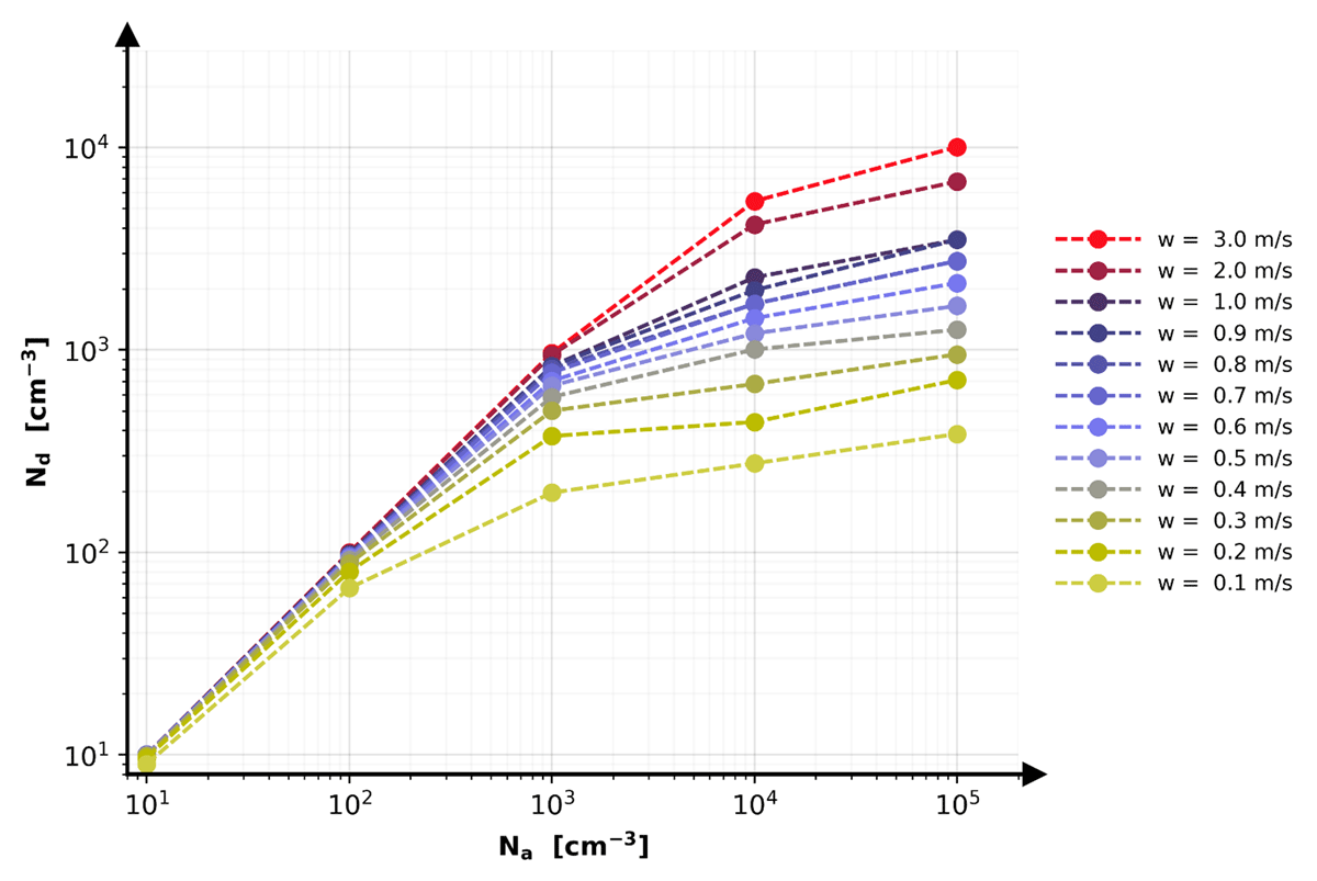
Figure 1
Parcel model simulations for different updraft speeds (in color) using PYRCEL. Each point represents one simulation. The droplet number concentration Nd as a function of the initial aerosol number concentration Na where Nd is diagnosed at the end of the model evaluation after the parcel is lifted for 2500 m. Particles are defined as cloud drops when their at the end of the simulation is larger than their at the point of maximum supersaturation.
3.2. Base case evaluation
Before we evaluate the susceptibility response in MIMICA, we compare our results with those from the LES intercomparison study conducted by AM09. Figure 2 shows snapshots of LWP after two hours of simulation for different cases. MIMICA produces substantial precipitation during the first hour of simulation for low values of Na, but reaches a quasi-stationary state after this, without much precipitation. Qualitatively, the typical stratocumulus patterns observed from satellites and in other high-resolution models are captured by MIMICA, both on the LRD and SMD domains and for various choices of Na. Figure 3 shows a comparison of the time evolution of the LWP for all MIMICA simulations against the results of AM09. In general, the simulated evolution of the LWP using MIMICA compares well with the results from the AM09 LES intercomparison (especially the MIMICA simulations with Na = 65 cm–3 which should be comparable to AM09). However, our simulations—and especially those with higher aerosol loading—tend to produce lower LWP values at the end of the simulations compared to the results of AM09. We relate this characteristic to the fact that most models in AM09 used fixed Nd values, which leads to higher LWPs compared to when using prognostic Nd (cf. Bulatovic et al., 2019). Further exploring the LWP response to different aerosol loadings would be interesting but is not the main focus of this paper.
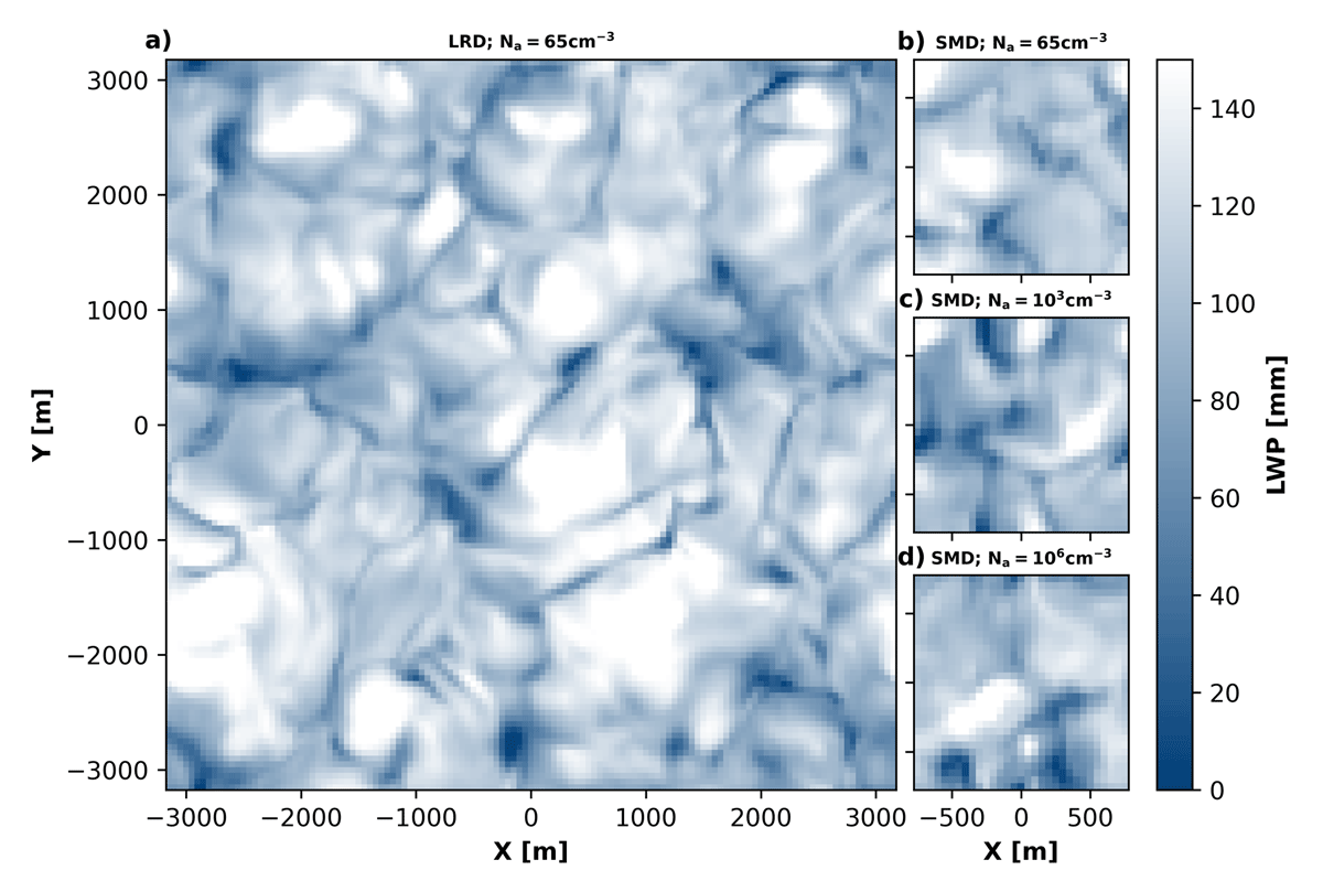
Figure 2
Liquid water path (LWP) after two hours of simulation for cases with on the LRD (a) and SMD (b, c, d) domains. In panel a) and (b) Na = 65 cm–3 while in panel (c) Na = 103 cm–3 and panel (d) Na = 105 cm–3.
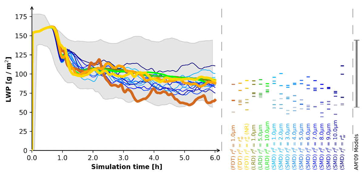
Figure 3
Comparison of liquid water path (LWP) between all our simulations with MIMICA (in color) and the simulations from Ackerman et al. (2009) in grey shading. The left panel shows the temporal evolution of the LWP for sensitivity simulations with aerosol number concentration Na = 65 cm–3. Each color corresponds to a specific sensitivity simulation, see text at the bottom of the central panel and main text for a description of the different sensitivity simulations. The central panel shows the LWP at the end of all sensitivity simulations with varying Na = {65, 100, 500, 103, 104, 105} cm–3 simulation (more transparent lines in the indicate higher Na). The right panel shows the range of simulated LWP by Ackerman et al. (2009).
Figure 4 shows a comparison between the simulated profiles of updraft variance, cloud droplet number, total water content, and liquid water content. For the updraft variance (Figure 4a), all of our simulations have a maximum updraft variance between 0.1–0.4 m2s–2, which roughly corresponds to a typical updraft strength (expressed in terms of updraft standard deviations) of 0.3–0.6 ms–1. According to our parcel model simulations (cf., Figure 1), such updraft strengths should lead to a leveling-off of Nd at maximum Na ≈ 1000–2000 cm–3.
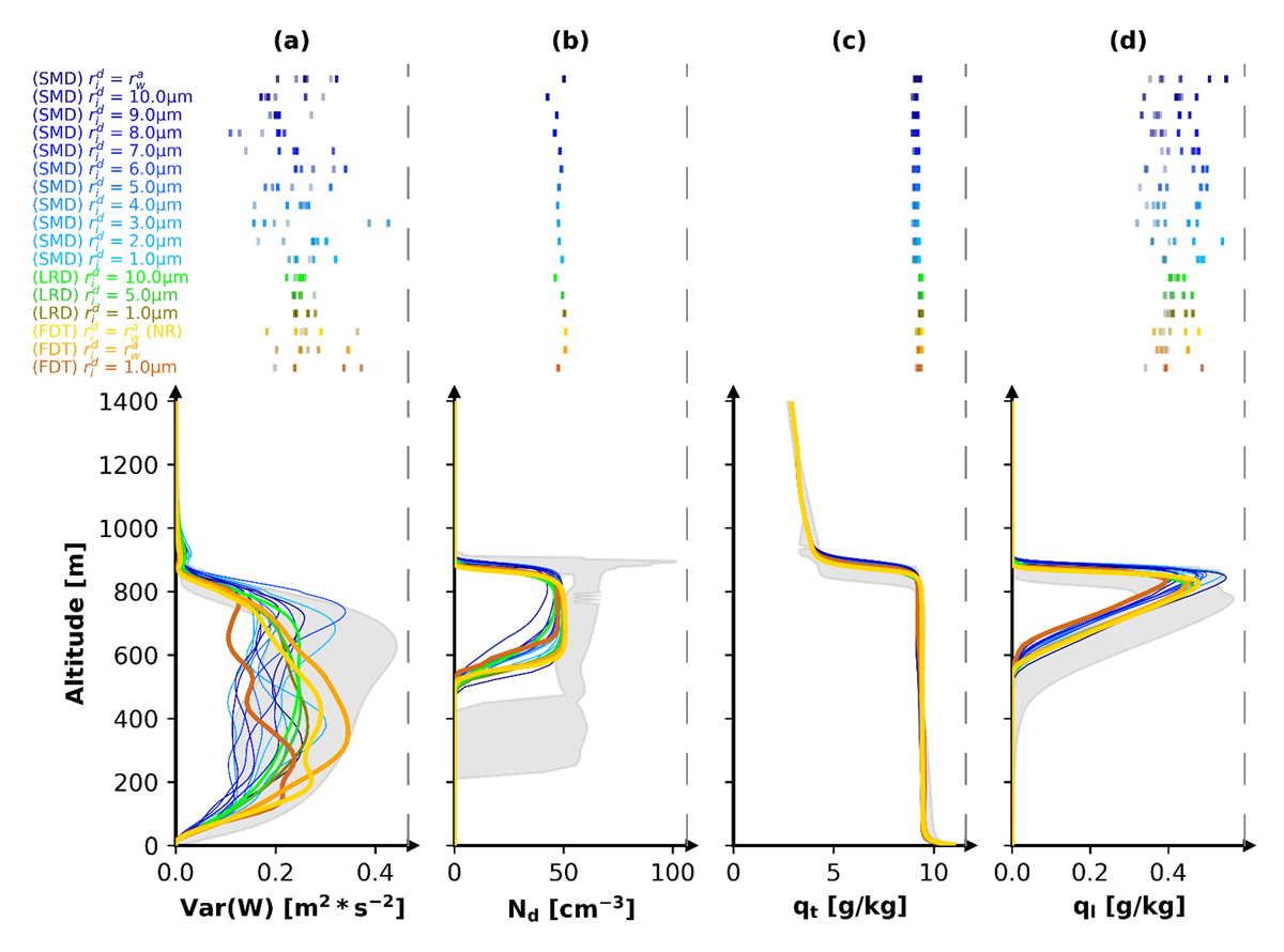
Figure 4
Modeled updraft variance (a), cloud droplet number Nd (b), total water content (c), and liquid water content (d) at the last modeled timestep. The upper row shows the maximum (median in panel c) value of the respective variable for all sensitivity simulations with MIMICA with varying aerosol number concentration Na = {65, 100, 500, 103, 104, 105} cm–3. Please see main text for a description of the different simulations. More transparent color indicates higher prescribed aerosol concentrations. The lower row shows profiles at the end of our simulations with Na = 65 cm–3 (colored lines). Gray shading indicates the modeled range (min/max) of the respective variable from the Ackerman et al. (2009) LES intercomparison.
The simulated Nd profiles in Figure 4b show an approximately constant Nd concentration within the cloud resulting from the homogeneous mixing assumption mentioned in Section 2.2. For the simulations with Na = 65 cm–3, we find Nd ≈ 50 cm–3, which is at the lower end of the simulated range of AM09. The cloud top altitude is approximately constant in all our simulations, while the cloud base is roughly 100 m higher than in AM09, leading to a thinner cloud geometric depth compared to the AM09 simulations. For total water (Figure 4c) and liquid water (Figure 4d) content, the simulated profiles agree very well with AM09.
3.3. Susceptibility simulations
Figure 5 shows the susceptibility simulations produced by MIMICA for the different setups outlined in Section 3.3.
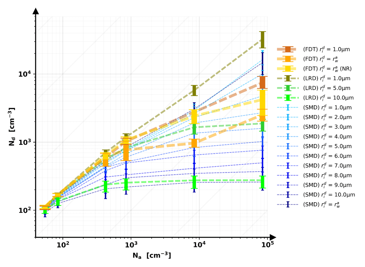
Figure 5
Susceptibility of in-cloud (ql > 0.1 g⁄kg) cloud droplet number concentration (Nd) to below cloud aerosol concentration (Na). Each point represents statistics from one simulation obtained from 3D MIMICA model output during the last of six hours of simulation. The error bars indicate the 25th and 75th percentiles. Blue lines show simulations on the small model domain (SMD) and darker blue colors indicate a larger initial droplet radius . Green lines show simulations on the large domain (LRD). Simulations with prescribed timestep (Δt = 0.1 s) are labeled FDT. All other simulations have time steps dictated by the CFL criterion. The orange, yellow and dark blue lines show simulations with initial droplet radius estimated from the wet aerosol PSD .
In the default setup of the model, the initial droplet radius of newly activated cloud droplets is assumed to be and the LRD is used. The corresponding (dark-green) line in Figure 5 shows that even at very high aerosol concentrations (reaching Na = 105 cm–3), a leveling-off of the susceptibility curve and hence a transition to the updraft-limited susceptibility regime is not generated by the model. It is worthwhile noting that there are some fundamental differences between a parcel and a large-eddy model that may affect the simulation results and the susceptibility curves. For example, the parcel model does not consider entrainment. In a subtropical stratocumulus cloud, with a drier free troposphere than the boundary layer, entrainment primarily occurs at cloud top and contributes to a drying of the boundary layer. Such a drying of the boundary layer could lead to an earlier onset of the regime shift from aerosol- to updraft-limited activation. However, we do not see any reason that entrainment effects, or any other structural differences between a large-eddy and a parcel model, should result in a complete absence of the updraft-limited regime in MIMICA.
A leveling-off of the susceptibility curve simulated by MIMICA is only visible when is increased to higher values (around 4–5 μm, cf. blue lines in Figure 5, which display simulations using the SMD setup for ranging from ). However, a necessary condition to obtain the leveling-off is that we use the renormalization procedure following Reisin et al. (1996) during activation (see Section 2.2, results not shown without renormalization). Figure 5 also shows that the choice of domain size (LRD vs. SMD) does not affect our conclusions (blue lines vs. green lines for ).
In general, the susceptibility curve starts to level off at lower Nd values as increases. This is expected as a larger initial droplet size consumes more water vapor and hence—due to the renormalization procedure—less supersaturated water is available to activate aerosols. Figure 6 shows supersaturation statistics (after the microphysical timestep; cf., Section 2.2) for simulations with Na = {65, 103, 105} cm–3. For simulations with higher aerosol loading, the modeled supersaturation decreases (note the different y-axis in the upper panels of Figure 6), while there is little difference in the supersaturation statistics between the simulations with a similar aerosol load. Note, however, that the 99th percentile values decrease with increasing and that the fraction of supersaturated grid boxed (fRH; defined as the fraction between the number of pixels with RH > 100 and all pixels) decreases for simulations with larger as shown in the lower panels of Figure 6. For example, in the SMD simulations with a high aerosol load of Na = 105 cm–3 (blue boxes in Figure 6c), the fraction of supersaturated grid points when assuming is compared to when assuming .
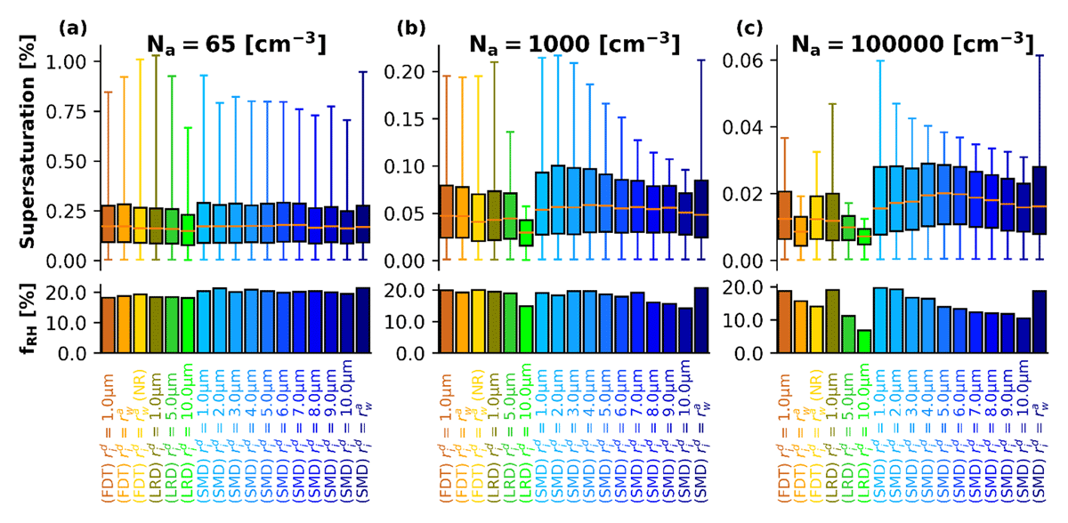
Figure 6
Supersaturation statistics for simulations with Na = {65, 1000, and 10000} [cm–3] (left, middle and right panel respectively). The statistics are obtained from the 3D output at the last model time step. The barplots (lower panels) indicate the fraction of supersaturated grid boxes (fRH) within the domain. The boxplots (upper panels) show the 25th and 75th percentiles (boxes) and 1st and 99th percentiles (whiskers) of supersaturation of all supersaturated gird boxes. Please note the different y-axes.
To test if MIMICA can simulate the transition to the updraft-limited activation regime with a smaller timestep, we conducted a set of susceptibility simulations with a prescribed timestep of Δt = 0.1s using the SMD setup with (with the renormalization procedure on; light brown line in Figure 5). At high aerosol concentrations (Na ≥ 103 cm–3), the susceptibility curve shows some leveling-off. However, the leveling-off arguably happens at higher Nd levels compared to the parcel model simulations with similar conditions (cf., Reutter et al., 2009 and Figure 1). In contrast, the susceptibility simulations with a small time step (Δt = 0.1s, FDT) and with calculated from integration of the PDF of the wet aerosol size distribution (with the renormalization procedure on; orange line in Figure 5) lead to a leveling-off at round Nd ≈ 400 cm–3 for Na = 104 cm–3, which is consistent with the results from the parcel model. However, Nd then increases again at Na = 105 cm–3, which is unexpected. We speculate that an even smaller time-step is necessary to accurately simulate activation at these high aerosol concentrations. A leveling off is also visible when we use a small time step (Δt = 0.1s) together with from the wet aerosol PSD but without the renormalization procedure described in Section 2.2 (simulation labeled NR, yellow line). The observed Nd for this simulation fall between the values reached in the simulations with an assumed and those where the wet radius was used together with the renormalization procedure. Additionally, we also tested if we could reproduce the leveling-off using and the larger time step (Δt ≈ 2s) dictated by the CFL-criterion but these simulations (darkest blue line in Figure 5) do not show any leveling off.
4. Discussion and Conclusions
We have investigated if a large-eddy model with explicit aerosol-cloud interactions and a widely used two-moment bulk microphysics scheme (Seifert and Beheng, 2001, 2006) can reproduce the cloud droplet susceptibility regimes identified by Reutter et al. (2009) for a warm stratocumulus cloud, i.e. the aerosol-limited (β ≈ 1) and updraft-limited regime (β ≈ 0), respectively. Accurately simulating these susceptibility regimes, and in particular the updraft-limited regime, is an important necessity for several reasons: First, the two regimes have frequently been identified in observations, at different geographical locations and for different cloud types (e.g., Bougiatioti et al., 2016; Bougiatioti et al., 2020; Georgakaki et al., 2021; Guy et al., 2021;Hudson and Noble, 2014; Kacarab et al., 2020; Misumi et al., 2022). Second, Sullivan et al. (2016) used global climate model output to show that updraft velocity fluctuations can explain a substantial fraction of the temporal evolution of Nd, i.e., the updraft-limited regime may dominate on a global scale in climate models. Third, in well-mixed boundary layers, where up- and downdrafts approximately balance each other, there will always be regions with low updrafts where Nd may be updraft-limited, which will impact the bulk susceptibility. Fourth, the onset of the transition between the aerosol-limited and updraft-limited regime leads to a flattening of the susceptibility curve well before the updraft-limited regime is reached; for an updraft <1 ms–1 (typical for a stratocumulus cloud), β is <1 already at Na < 1000 cm–3.
In the standard setup, the bulk microphysical scheme used here cannot simulate the transition from the aerosol- to the updraft-limited regime, which means that the model would overestimate the susceptibility at high aerosol number concentrations or low updrafts. Only when implementing a renormalization procedure following Reisin et al. (1996), which limits the amount of water vapor available for condensational growth, and at the same time, increasing the initial droplet radius of newly activated droplets to values larger than , a regime transition emerges. However, a clear recommendation for cannot be made upon physical arguments at this point. A pragmatic solution to the problem can be to simply consider as a tuning parameter. Seifert and Beheng (2006) originally suggested to (arbitrarily) assume a mass of mi = 1 × 10–12 kg for newly formed droplets, which would correspond to . Our sensitivity studies show that using leads to a reasonable transition in the susceptibility regimes for the considered meteorological setup. However, such a large is quite unphysical as it takes several seconds for a cloud droplet to grow to such size, i.e., longer than the typical timestep of a Large-Eddy Model, and it may not be recommended to use such an approach when aiming to study processes related to aerosol-cloud interactions (see Loftus, 2018). A more reasonable choice is to estimate from integrating the wet aerosol PSD as outlined by, e.g., Khvorostyanov and Curry (2006). This approach, however, only gives reasonable results when the time step is small enough (Δt ≈ 0.1s).
Árnason and Brown (1971) pointed out that the timestep to resolve the rate at which a droplet population responds to changes in supersaturation decreases as the number concentration of droplets increases. Our results show that using a time step which is dictated by the dynamic CFL-criterion (Δt ≈ 2s together with the pseudo-analytic formulation used to estimate local supersaturation (Morrison et al., 2005; Morrison and Grabowski, 2008) is not sufficient to explicitly resolve the microphysical processes, which are responsible for the transition in the susceptibility regimes, in particular for heavily polluted conditions. A related issue is that we only see a reasonable transition between the susceptibility regimes when we limit the number of activated aerosols by the renormalization scheme described in Section 2.2. Not limiting the absolute number of activated droplets might be acceptable for models with very small timesteps (O(10 ms)), i.e., such models may be capable of accurately resolving the balance between supersaturation increases from adiabatic lifting and supersaturation depletion from activation and growth of hydrometeors. Not applying the renormalization could lead to an unphysical behavior in that the activated drops consume more supersaturated water vapor than available in a grid box.
LES models with bin-microphysics and a sufficient number of aerosol and hydrometeor bins should, in principle, be able to explicitly simulate the aerosol susceptibility regimes provided that they use a sufficient number of bins and small enough time steps (see Khain et al., 2015). A Lagrangian ’superdroplet’ parameterization embedded in the LES would also be a valid approach (Shima et al., 2009). Another potential solution to the abovementioned problems could be to implement a sub-time-stepping scheme with a microphysically defined sub-timestep which allows explicit calculation of the delicate supersaturation balance, e.g., as in Ong et al. (2022) or Tonttila et al. (2017). This is, however, beyond the scope of this study.
We want to note at this point that caution should be exercised when using LES or cloud-resolving models for the development of new parameterizations for global models (e.g., Glassmeier et al., 2019), or when using them in super-parameterized models (Grabowski, 2016), as it is by no means guaranteed that all LES can capture all relevant microphysical processes as shown in our analysis. Interestingly, global models should not be exposed to the problems described above as their aerosol-cloud interactions are fully parameterized. Advanced activation schemes, e.g., the one from Morales Betancourt and Nenes (2014), which take into account kinetic limitations during activation (Nenes et al., 2001), should be able to capture the transition in the susceptibility regimes as they are developed based on parcel model simulations, which can explicitly simulate the regime transition.
Data Accessibility Statement
All data analyzed in this study is available via the Bolin center data hub: https://github.com/matschwa/2023-LES-susceptibility/.
Code Availability
The code for the data analysis is available via github:https://github.com/matschwa/2022-LES-susceptibility.
The MIMICA model code is available upon request from Annica Ekman.
Acknowledgements
We would like to thank Rahul Ranjan, Ilona Riipinen, Frida Bender and Alejandro Baró Pérez for valuable discussions. We also thank Fabian Hoffmann for advice on the time step issue.
Matthias Brakebusch (ACES) and Hamish Struthers (NSC) are acknowledged for assistance concerning technical and implementational aspects in making the code run on the NSC resources. We acknowledge Daniel Rothenberg for making available PYRCEL via github (https://github.com/darothen/pyrcel).
Funding Information
This project has received funding from the European Union’s Horizon 2020 research and innovation program under grant agreement No 821205 (FORCeS) and the Swedish Research Council (2020–04158).
The computations and data handling were enabled by resources provided by the Swedish National Infrastructure for Computing (SNIC) at the National Supercomputer Centre (NSC), partially funded by the Swedish Research Council through grant agreement no. 2018–05973.
Competing Interests
The authors have no competing interests to declare.
Author Contributions
All authors participated in the design of the study. MS conducted all simulations and data analysis. MS & AE conceived and refined the overall structure of the investigation based on discussions with and feedback from all co-authors. MS drafted the manuscript with input from all co-authors. All authors have read and agreed to the published version of the manuscript.