Relation Between High-Pressure Blocking and Aerosol Concentrations in Southern Sweden

1 Introduction

It is common knowledge that Earth’s increasing temperature has many side effects. One such effect is the increase in frequency of extreme weather phenomena (Mitchell et al., 2006, Caupa & Rahmstrorf, 2023). One such phenomenon, which lacks extensive research, is high-pressure blocking events. A high-pressure blocking event is an anticyclone that covers an area for a prolonged period of time and often blocks other types of weather, hence the name. This results in limited cloud formation and pronounced daily temperature variations (Lupo, 2021). Furthermore, anticyclones are also associated with slower air movement, causing the air to remain stagnant. This can lead to an accumulation of air pollutants such as aerosols (Jacob, 1999).

Anticyclones are meteorological high-pressure systems in which air sinks toward the ground, creating a region of high pressure (Spiridonov & Mladjen, 2021). The descending air undergoes adiabatic compression, which results in an increase in air temperature. This temperature increase inhibits cloud formation, as warmer air can hold more moisture. The absence of clouds leads to a large temperature difference between day and night, with summer anticyclones being associated with high temperatures and winter anticyclones with low temperatures. Anticyclones are generally associated with cloud-free weather but can cause low lying stratus clouds, and even light precipitation, during winter. Due to the Coriolis force the winds during anticyclones rotate in a clockwise direction in the Northern Hemisphere.

A high-pressure blocking period refers to a prolonged anticyclone characterised by higher surface pressure covering a large area (Lupo, 2021). Since blocking events extends over a vast region, the pressure gradient remains small due to minimal pressure fluctuations. As a result, the wind tends to be calm. A blocking period is typically defined as lasting between five and ten days, although some events can persist even longer (Porebska & Zdunek, 2013). However, no single definition of high-pressure blocking events exists (Lupo, 2021). High-pressure blocking events are often followed by precipitation and/or a strong shift in wind direction.

Lupo (2021) showed that the frequency of high-pressure blocking periods has increased in the Northern Hemisphere, including Europe, during the last 50 years. Luo, Yao, and Dai (2015) found that high-pressure blocking events were more common in eastern Europe during 1978 to 1994, and more common in western Europe during 1995 to 2001. Fahimi et al. (2020) investigated high-pressure blockings over the Atlantic Ocean, Europe and Western Asia and showed that although high-pressure blocking events decreased between 1959 to 1988, they increased from 1989 to 2011. Rutgersson et al. (2022) summarised existing knowledge regarding extreme events in the Baltic area, including high-pressure blockings. They found that some research such as that of Coumou, D., Lehmann, J. and Beckmann, J. (2015), and Francis and Vavrus (2015), indicate that the Baltic area should experience an increase in the frequency of high-pressure blocking due to decreased temperature gradients associated with Arctic amplification. But Rutgersson et al. (2022) also highlight that the link between Arctic amplification and wavier circulation at mid-latitude (resulting in more blocking events) has been questioned (Blackport & Screen, 2020). Furthermore, a review of blocking frequencies by Woollings et al. (2018) found that trends regarding changes in high-pressure blockings are very sensitive to the choice of the definition of the blocking.

Weather patterns in general and anticyclones in particular can be classified by using different kinds of classifications (Philipp et al., 2010). One such classification is the Hess and Brezowsky macrocirculation types (1952) in which anti-cyclonic weather is categorised into several sub-categories. Three such anticyclonic patterns that often impact the weather in Scandinavia are the Fennoscandian High (HFA), the Southeast Anticyclone (SEA), and the Central European High (HM) (Bartholy, Pongracz & Pattantyús-Ábrahám, 2006). Another weather pattern classification is the Lamb weather type (LWT), which classifies circulation types due to the wind direction and type of flow (Lamb, 1972). This approach has been applied in a study linking meteorological conditions to pollen and air pollution concentrations in southern Sweden (Grundström et al., 2017). In the LWT categorisation, circulation types are grouped as anticyclonic (A), cyclonic (C), and directional (N, NE, E, SE, S, SW, W, NW), as well as hybrid forms that combine pressure regime and flow direction. For example, AW, ANE, and ASE represent anticyclonic conditions associated with westerly, north-easterly, and south-easterly airflows (Grundström et al., 2017).

During an anticyclone, adiabatic compression of the air occurs as the air descends. This increases the temperature at lower altitudes. However, this downward movement of air does not reach the ground due to the friction opposed by buildings, forests, valleys, and other obstacles that create friction by disrupting the airflow (Lautrup, 2011). Thus, the downward draught will spread out a few hundred meters above the ground and not mix with the air that lies closest to the ground. Since the air closest to the ground remains cool, while the air a few hundred meters up is warmer from the adiabatic compression, an inversion of the environmental lapse rate will be created. This is called a subsidence inversion and will prevent air mixing between the ground level and the upper layers of the atmosphere (Gramsch et al., 2014).

The absence of clouds during the anticyclone also promotes ground inversions during night-time. Outgoing radiation from the Earth causes a strong cooling of the surface which in turn cools the air closest to the ground. This creates a ground inversion layer, where the air temperature increases with height in the lowest atmospheric layers (O’Hare, Wilby & Sweeney, 2005). Crétat et al. (2024) have shown that the topography and imperviousness of the surrounding area has a large influence on ground inversions. Urban locations are linked to stronger ground inversions due to impervious surfaces and reduced air circulation, whereas forested areas typically have weaker inversions because of canopy shading and enhanced air mixing. During the day, the air in the boundary layer is well mixed, but during the night the surface is cut off from the layer above the inversion, the residual layer (Wallace & Hobbs, 2006). Vertical air movements are inhibited until early morning, when solar heating breaks up the inversion and mix the air from the residual layer from the previous day with the air closer to the surface.

Aerosol particles can substantially impact both climate and human health. Aerosol particles have a range of sources and their lifetime in the troposphere is approximately one week (Balkanski et al., 1993). This means that they can be transported from region to region and from one country to another. During this transport, formation of aerosol from gaseous compounds and chemical transformation of existing particles can occur. Aerosol particles come in a range of sizes from a few nanometres up to several micrometres. When dealing with aerosols it is important to specify which types and sizes of particles are being measured, where PM2.5 (particulate matter with an aerodynamic diameter of 2.5 µm or less) is a common choice. Although aerosols can form naturally in the atmosphere, the primary sources in urban and suburban Europe include solid fuel combustion for domestic heating, industrial activities, and road transportation (European Environment Agency, 2024). Particulate contributors to PM2.5 include sulfuric acid (SO₄) and soot (black carbon), both originating from the burning of fossil fuels.

Studies have demonstrated a correlation between elevated PM2.5 concentrations and an increased risk of respiratory, cardiovascular, and cerebrovascular diseases, as well as diabetes (Sharma, Chandra, & Kota, 2020). Sommar et al. (2021) showed in a cohort study of the large Swedish cities of Gothenburg, Stockholm and Umeå that PM2.5 has a direct negative influence on human health. This study showed that for every 5 µgm^–3 increase in PM2.5 concentrations, the natural mortality rise with 13%. Furthermore, the risk of cardiovascular dieses also increases with PM2.5. Ljungman et al. (2019) showed that PM2.5 from residential heating was linked to a higher risk of ischemic heart disease and that black carbon increased the risk of stroke. Thus, there is strong evidence that an increase in PM2.5 will have a direct negative impact on the health of the people in the region. In 2008, the European Union set an annual mean limit value for PM2.5 concentrations at 25 µgm^–3, although the WHO suggested a much lower threshold of only 5 µgm^–3 (European Parlament and Council, 2024). In 2030, a new limit value of 10 µgm^–3 will replace the old limit value (European Parliament and Council, 2024). In 2022, the EU current mean limit threshold was exceeded in several European countries, including Croatia, Bosnia and Herzegovina, Italy, Poland, North Macedonia, and Türkiye (European Environment Agency, 2024).

During a high-pressure blocking event the environmental lapse inversion, especially the subsidence inversion, prohibits vertical air mixing in the atmospheric layers closest to the ground. If aerosols are produced at ground level during this high-pressure blocking event, the aerosols would not disperse vertically, implying higher concentrations at ground levels. Thus, one would expect higher concentrations of PM2.5 during high-pressure blocking events. Different studies, such as Dempsey (2018) in Ontario, Canada; Messori et al. (2018) in Europe; Shin et al. (2021) in Seoul, Korea; and Özdemir, Birinci, and Deniz (2024) in Istanbul, Türkiye, all correlated regional high-pressure blocking events with increased concentrations of PM2.5. The reasons for the increases include less vertical dispersion of aerosols during the events, stagnant air conditions, and shifted air movements.

Grundström et al. (2017) linked different LWT circulation types with increases in birch pollen and also PM10 by examining the airflow in Gothenburg and Malmö. The results showed an increase in high-level aerosol events in Malmö with the circulation type SE, indicating advection from higher emission areas. However, this study did not account for hybrid forms, such as anticyclonic conditions combined with SE, which should work together to increase the aerosol levels in Malmö. As aerosol emissions are particularly high in central European countries (European Environment Agency, 2024), anticyclonic winds from the south and east from AS, ASE, and AE are expected to increase PM2.5 concentrations in southern Sweden. These aerosols would be transported to southern Sweden via southerly to easterly winds during the anticyclone.

In this study we investigate how the concentrations of aerosol particles change during high-pressure blocking events in southern Sweden. We used meteorological data from the Swedish Meteorological and hydrological institute (SMHI) to determine periods of high-pressure blocking events and analysed the PM2.5 levels in a rural (Vavihill, Svalöv, Skåne County) and an urban (Malmö, Skåne County) location during the high-pressure blockings. Wind direction, season, and the average pressure during the events were used to gain a comprehensive understanding of how PM2.5 levels change under different types of high-pressure blocking events. In this study we also explore the long-term frequency of high-pressure blocking events in southern Sweden to determine whether this weather phenomenon is becoming more common here, which is particularly important if a positive correlation with aerosol levels is found.

2 Method

2.1 The data handling and devices

The meteorological data was downloaded from the SMHI website. The data included hourly atmospheric pressure data, hourly precipitation data, and hourly wind data (speed and direction). Aerosol data as PM2.5, measured over one-hour intervals, was also downloaded. One urban and one rural site were selected. The locations were chosen based on their classification as rural or urban and the length of time the stations had been in operation, using the duration of the time series as a criterion.

2.1.1 The aerosol data and measurements

The rural measuring station in the county of Skåne with the longest aerosol time series was Vavihill, located in Svalöv municipality, southern Sweden. This station was active from September 28, 1999, to November 15, 2017. However, only 57% of the period contained non-missing values. Additionally, between 2017 and 2018, the Vavihill station was relocated to nearby Hallahus, where we have acquired data from the 10th of May 2018 to the 31st of December 2022. For this period, 93% of the data was non-missing values. Combining these two datasets resulted in a total of 5371 days of hourly data. For an urban location in the county of Skåne, Malmö Rådhuset had the longest aerosol time series. The measurement series there went from the 3rd of June 1999 to the 31st of December 2023. Here, 90% of the recorded values were non-missing, resulting in 8074 days of data. The geographical location of the two stations, together with pictures showing the surrounding area, can be seen in Figure 1. The PM2.5 measurement device used at Vavihill and Malmö can be seen in Table 1.

Table 1

The PM2.5 measurement device for each location.

STATION	PERIOD	DEVICE	PRECISION (± µG/M–)	NOTE
Vavihill	28-09-1999 to 15-11-2017	TEOM 1400	1.5
	10-05-2018 to 31-12-2022	Palas FIDAS 200	0.1
Malmö	03-06-1999 to 01-01-2009	TEOM 1400	1.5
	01-01-2009 to 31-12-2015	TEOM 1400 + FDMS 8500 B/CB dryer	1.5	Combined system with dryer unit
	01-01-2016 to 31-12-2021	TEOM 1405F + FDMS 8500 B	2	Combined system with dryer unit
	01-01-2022 to 31-12-2023	Palas FIDAS 200	0.1

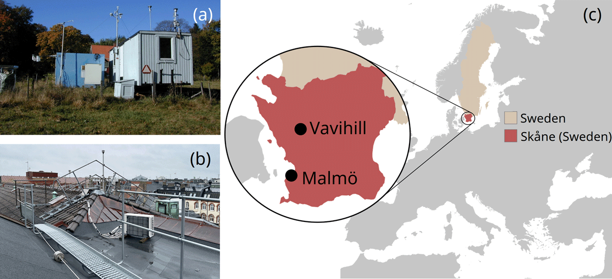
Figure 1

2.1.2 The meteorological data and measurements

The meteorological data used in this study can be observed in Table 2. The time periods listed in the table show those used this study, which may not represent the full operational range of the stations. The choice of meteorological data was based on the proximity to the PM2.5 measuring stations in the case for Vavihill and Malmö and on the availability of data covering as much of the PM2.5 measurements as possible. For Vavihill, there were no meteorological measurements nearby the station. The pressure data used for Vavihill was therefore data from Helsingborg, 25 km away. However, Helsingborg is a coastal city and can experience daily cycles of sea breezes and land breezes and we therefore chose precipitation and wind data from Hörby (35 km from Vavihill), which is situated more inland.

Table 2

The meteorological data for each location.

		VAVIHILL	MALMÖ	ÄNGELHOLM
Air Pressure	Station	Helsingborg (25 km away from particle monitor)	Helsingborg (49 km away from particle monitor)	Ängelholm airport
	Period	01-08-1995 to 01-10-2024	02-08-1995 to 01-10-2024	05-01-1946 to 01-10-2024
	Device	Vaisala PTB220 (15-04-2015 to 17-04-2025 and from 19-09-2004 to 23-05-2014) PTB201A (Remaining time).	Vaisala PTB220 (15-04-2015 to 17-04-2025 and from 19-09-2004 to 23-05-2014) PTB201A (Remaining time).	No information
Wind	Station	Hörby (35 km away from particle monitor)	Malmö (6 km away from particle monitor)	Ängelholm airport
	Period	01-08-1995 to 01-10-2024	01-01-1990 to 01-12-2024	05-01-1946 to 01-03-2025
	Device	Vaisala WAA15A (speed) Vaisala WAV15A (direction)	Vaisala WAA15A (speed) Vaisala WAV15A (direction)	No info
Precipitation	Station	Hörby (35 km away from particle monitor)	Malmö (6 km away from particle monitor)	Ängelholm airport and Tånga.
	Period	01-08-1995 to 01-10-2024	21-11-1995 to 01-12-2024	18-01-1947 to 30-11-2001 (Ängelhom airport), and 19-12-1973 to 31-08-2024 (Tånga).
	Device	Geonor T200	Geonor T200	No information and beaker.

For Malmö, both wind and precipitation data from the city are used but the pressure data was not available from this measurement station for the entire PM2.5 measurements period. Pressure data from Helsingborg was therefore also used for the PM2.5 measurements from Malmö. During high-pressure blocking events there are very small variations in pressure; using pressure data from a station some distance away was therefore evaluated not to constitute a problem in the present work. For example, during the period from December 1st, 1995, to October 1st, 2024, the mean difference in pressure between Ängelholm and Helsingborg was (0.25 ± 0.20) hPa, indicating a very small difference.

For the analysis of whether high-pressure blockings have become more common we wanted a time series that was as long as possible. We therefore used data from Ängelholm airport, which has hourly pressure measurements from 1946 to present day. Precipitation data from Ängelholm airport was used in conjunction with the nearby station of Tånga. This was utilised as the precipitation data from Ängelholm did not cover the entire period, so Tånga was used to cover the time periods that Ängelholm airport lacked (see Table 2).

2.2 The identification of high-pressure blocking events

To evaluate the occurrence of high-pressure blocking event for Vavihill or Malmö, the precipitation data and atmospheric air pressure were used, which can be seen in Figure 2. For a period to be defined as a high-pressure event, the atmospheric pressure had to be over 1014 hPa for at least 5 days. This time period was chosen since a five-day limit is often considered when classifying high-pressure blocking events (Lupo, 2021). A pressure limit of 1014 hPa was chosen as this was the median atmospheric pressure in Helsingborg during the measurement period. During the investigation of the data, we found that extended periods with steady higher pressures generally had lower absolute pressure values during summer than during winter. To ensure that we did not get a seasonal bias in the determination of blocking events we therefore settled on a limit in which the pressure would be higher than the median value at the station.

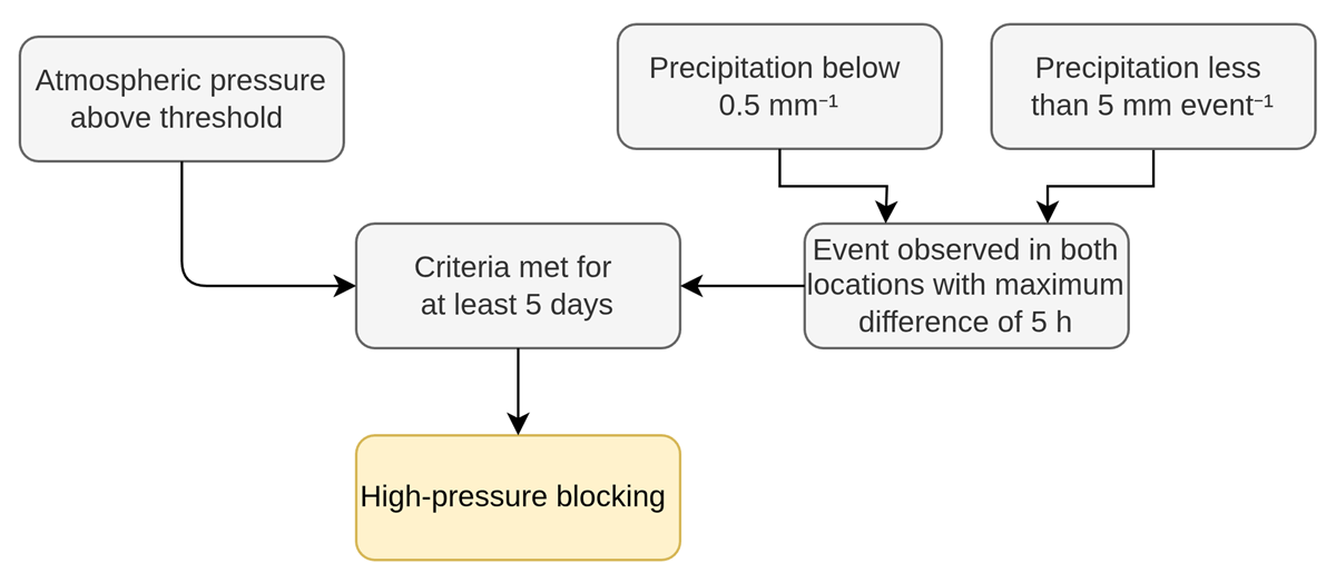
Figure 2

To ensure that only periods of extended high-pressure weather were included, we also added a precipitation criterion for high-pressure events. As high pressure blocking events steer frontal activity away from the area and convective activity is limited by the subsidence, we expect very limited rain amounts and intensities during a high-pressure blocking event. The maximum hourly precipitation limit was set to 0.5 mmh^–¹ since it corresponds to light precipitation according to the Swedish Meteorological and Hydrological Institute (SMHI, 2011). Other studies, such as Sun et al. (2019), also used an upper limit of 0.5 mmh^–¹ to classify light precipitation. To avoid events with light precipitation for an extended period, an event limit of 10 hours of light precipitation was imposed. For this criterion, a maximum amount of accumulative precipitation of 5 mm cannot be exceeded during the entire event.

As a high-pressure blocking event covers a large geographical area, and Vavihill and Malmö are located close to each other, a blocking event observed at one location should also be detectable at the other. To account for this, all identified high-pressure blocking events at one location were required to correspond to an event at the other location within a maximum time difference of 5 hours. Furthermore, if the blocking event ended earlier at one location, the ending time at the other location was adjusted accordingly, with a maximum allowable difference of 5 hours. However, since Vavihill and Malmö used the same air pressure measuring station, this meant that the precipitation in both locations had to be under 0.5 mmh^–¹ and 5 mm for the event.

To evaluate the sensitivity of our results to the selection criteria for the pressure limits, we increased the minimum pressure threshold by 2 hPa, 4 hPa and 6 hPa. The number of events included in the analysis decreased by 36, 103, 163 for Vavihill and 34 99, 152 for Malmö. However, even with fewer events included in the analysis, the results presented in Section 3 regarding trends in PM2.5 concentrations during the events remain significant.

For the analysis on long-term changes in blocking frequency, the precipitation limit was set to 1 mmd^–¹ for the Ängelholm data as daily precipitation data was used for this station. This limit was chosen as it corresponds to 2 hours of light precipitation.

The thresholds used in this study follow the logic of established threshold-based circulation classification (THR) schemes such as LIT (Litynski advection and circulation types), LWT2 (Lamb-weather types version 2), and Schüepp (Alpine Weather Statistics) presented by Philipp et al. (2010). These classifications all rely on statistically defined thresholds, derived from the data in question. These include percentiles, standard-deviation-based ranges, or long-term means. As mentioned by Philipp et al. (2010), threshold choices always contain a subjective element, but the advantage is that they give reproducible and clear classifications. In the same way, the thresholds in this study are statistically defined, and physically meaningful. The thresholds in this study were chosen based on the data in question, together with the well-known characteristics of high-pressure blocking. Furthermore, the thresholds were varied to determine the sensitivity of the results.

3 Results

3.1 The change in aerosol concentrations

After applying the high-pressure blocking detection method to the data from Vavihill and Malmö for the entire period, a total of 226 high-pressure blocking events were identified between 1995 and 2024. A filter requiring 85% data coverage of PM2.5 data was applied to these blocking events. For Vavihill, 122 high-pressure blocking events were removed due to insufficient PM2.5 data, leaving 104 relevant high-pressure blocking events for the analysis. For Malmö, 52 high-pressure blocking events were removed due to insufficient PM2.5 data coverage, which resulted in 174 high-pressure blocking events being included in the analysis.

An example plot showing periods of high-pressure blocking events can be seen in Figure 3. This figure provides insight into the categorisation of high-pressure blocking events for the two different locations.

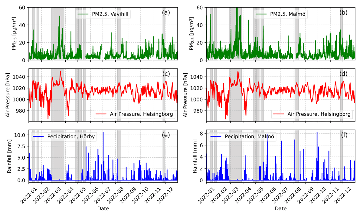
Figure 3

To evaluate the progression of aerosols levels during the evolution of the high-pressure blocking events, the mean and standard deviation PM2.5 levels were calculated for all the high-pressure blocking events for each hour since the start of each event. As the high-pressure blocking events varied in length, the number of events included in the event decrease after day 5 (Figure 4), but a minimum of eight events were required when calculating the mean and standard deviation of the PM2.5 data. The mean PM2.5 value is compared with the mean PM2.5 value during periods without high-pressure blocking events, as well as with the EU annual mean limit for PM2.5.

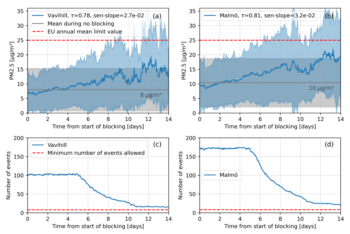
Figure 4

The average change in PM2.5 concentrations during periods of high-pressure blocking can be seen in Figure 4. The data is compared with the PM2.5 mean taken from periods without high-pressure blocking events. An increase in PM2.5 concentrations can be seen in Malmö from 10 µgm^–3 to a maximum of 22 µgm^–3 at day 13, and an increase from 7 µgm^–3 to a maximum of 19 µgm^–3 at day 12 can be seen in Vavihill. The increase is supported by the large τ-value of τ = 0.81 in Malmö, and τ = 0.78 in Vavihill. The Sen’s slope values also indicate a stronger increase in Malmö 3.2 × 10^–² µgm^–3d^–¹ compared with 2.7 × 10^–² µgm^–3d^–¹ in Vavihill. The decrease around day 10 can be attributed to the end of high-pressure blocking events that were associated with high PM2.5 levels.

To investigate if the PM2.5 levels returned to normal after the end of the events, the mean and standard deviation of the PM2.5 levels were also calculated from the end of each high-pressure blocking event and onwards. In Figure 5, one can observe that after the end of the high-pressure blocking events, the PM2.5 levels often drop to levels close to the average during the first day after the end of the event. This is an interesting result that highlights that the increase observed in Figure 4, is indeed due to the presence of a high-pressure blocking event. This drop after the event is expected since high-pressure blocking events are often terminated by frontal or low-pressure systems that result in precipitation. Precipitation is an efficient removal mechanism of pollutants in the air. The end of the blocking event is also often associated with a change of wind direction, increased wind speeds and a removal of the subsidence inversion. These factors together contribute to a fast decrease in aerosol concentrations.

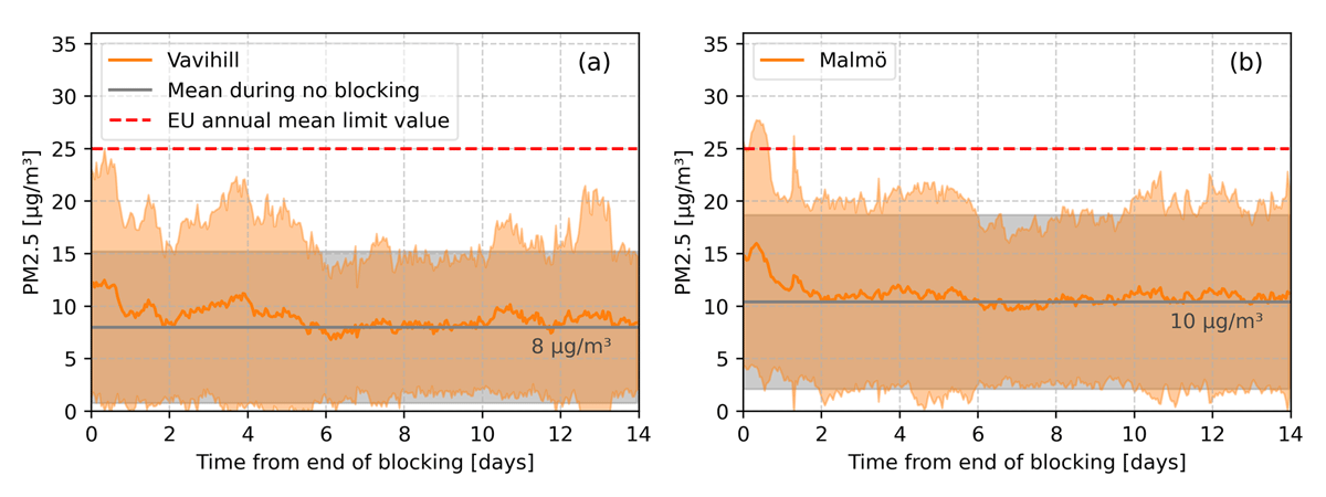
Figure 5

3.1.1 The change in aerosol concentrations depending on wind direction

The blocking events were sorted in different ways to explore how the PM2.5 concentration depended on different parameters. Firstly, the data was sorted into one of four wind categories: north-east (310° to 70°), south-east (70° to 190°), west (190° to 310°), and mixed direction. If 50% of the wind directional data fell into one of these categories, the event was assigned to that category (with zero wind speed being handled as a missing value). Cases in which no more than 50% of the data came from one single direction were categorised as mixed direction. These wind directions were chosen based on aerosol emission types and strength of sources. Higher relative anthropogenic aerosol emissions are observed in central and eastern Europe (European Environment Agency, 2024), and the south-east (70° to 190°) wind category was chosen to represent this direction. The westerly wind direction represents marine aerosol emissions in combination with some anthropogenic emissions from countries west and southwest of Skåne. The north-eastern category (310° to 70°) represents airmasses with general low aerosol levels from the Arctic and the regions north and northeast of Skåne.

The change in PM2.5 concentrations in Vavihill and Malmö during high-pressure blocking events for different wind directions can be seen in Figure 6. In the case of Vavihill, 9.6% of the winds came from the north-east, 23.1% from the south-east, 24.0% from the west and 43.3% from the mixed direction. For Malmö, 9.2% of the winds came from the north-east, 24.7% from the south-east, 21.8% from the west and 44.3% from the mixed direction. Very little data is observed from the north-east because this is an uncommon wind direction during high-pressure blocking events. A large proportion of the data was categorised as mixed, since high-pressure blockings are often not completely stationary and their movement results in changing wind directions.

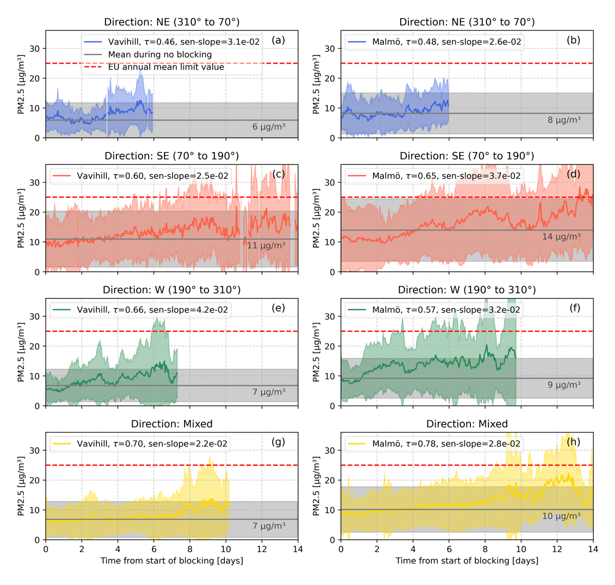
Figure 6

The changes in PM2.5 concentrations with winds from different directions can be seen in Figure 6. One can observe similarities between the aerosol concentrations depending on wind directions for Vavihill and Malmö, where a larger increase can be observed in Malmö. When only considering the north-east direction, no strong increase or high levels of PM2.5 were detected, as supported by the τ-values being under 0.5 for both Malmö and Vavihill Figures 6a & 6b. The southeastern wind direction displays the highest PM2.5 concentrations out of all directions. Vavihill yielded a τ-value of 0.60 and a maximum concentration of 22 µgm^–3 (Figure 6c). Malmö yielded a high τ-value of 0.65 and the mean concentration, for all blocking events from the south-east, exceed the EU annual mean limit value with a maximum concentration of 28 µgm^–3 (Figure 6d). For the western wind direction, an increase in PM2.5 can be seen in Vavihill as supported by τ = 0.66 (Figure 6e). The western wind direction for Malmö showed a similar increase. Although elevated levels can be seen on day nine, one must note that the spread of the values is large (Figure 6f). The mixed direction in Figures 6g & 7h showed increases similar to the increase in Figure 4. Also, when the wind direction is changing during the blocking events a monotonic increase is observed, supported by τ = 0.70 in Vavihill and τ = 0.78 in Malmö.

3.1.2 The change in aerosol concentrations depending on season

The data was also sorted according to the season when the blocking event occurred. As the amount of locally produced and transported anthropogenic aerosols depends on the season, it is of interest to investigate the PM2.5 trends for the different seasons separately. Furthermore, meteorological conditions also vary between the seasons. The categorisation was done by taking the midpoint date of the blocking and categorising the month it occupied into a season. December, January, and February were considered winter; March, April, and May were considered spring; June, July, and August were considered summer and September, October, and November were considered autumn.

The seasonal change in concentrations of PM2.5 during high-pressure blocking events can be seen in Figure 7. In Vavihill, 23.4% of the blocking events occurred during the winter, 29.9% during the spring, 20.8% during the summer and 26.0% during the autumn. In Malmö 23.5% of the blocking events occurred during the winter, 31.8% during the spring, 16.7% during the summer and 28.0% during the autumn. The average general concentrations (grey lines) show that the highest PM2.5 concentrations occur in winter and spring in Malmö and lower PM2.5 concentrations are observed during the summer in both locations. During the winter, a weak increase in the PM2.5 concentrations can be observed in Vavihill while Malmö has a much stronger increase, which is supported by τ = 0.66 and the Sen’s slope being 5.8 × 10^–² µgm^–3d^–¹ (Figure 7a & 7b). However, the average values for the winter plot in Vavihill ended 3 days before that in Malmö due to an insufficient number of events. In Malmö, the average values are almost at the EU annual mean limit value at day eight. A slight increase can be seen for spring in both locations, with Vavihill going from 9 µgm^–3 to a maximum of 13 µgm^–3, and Malmö from 11 µgm^–3 to a maximum of 18 µgm^–3 (Figure 7c & 7d). There are steady increases in PM2.5 levels during summer, although they start and end at much lower values than during the other seasons. A large increase can be seen during the autumn (Figure 7g & 7h), where high levels of PM2.5 can be observed towards the end of the period, with Vavihill going from 8 µgm^–3 to a maximum of 16 µgm^–3, and Malmö from 11 µgm^–3 to a maximum of 28 µgm^–3, which is above the EU annual mean limit value.

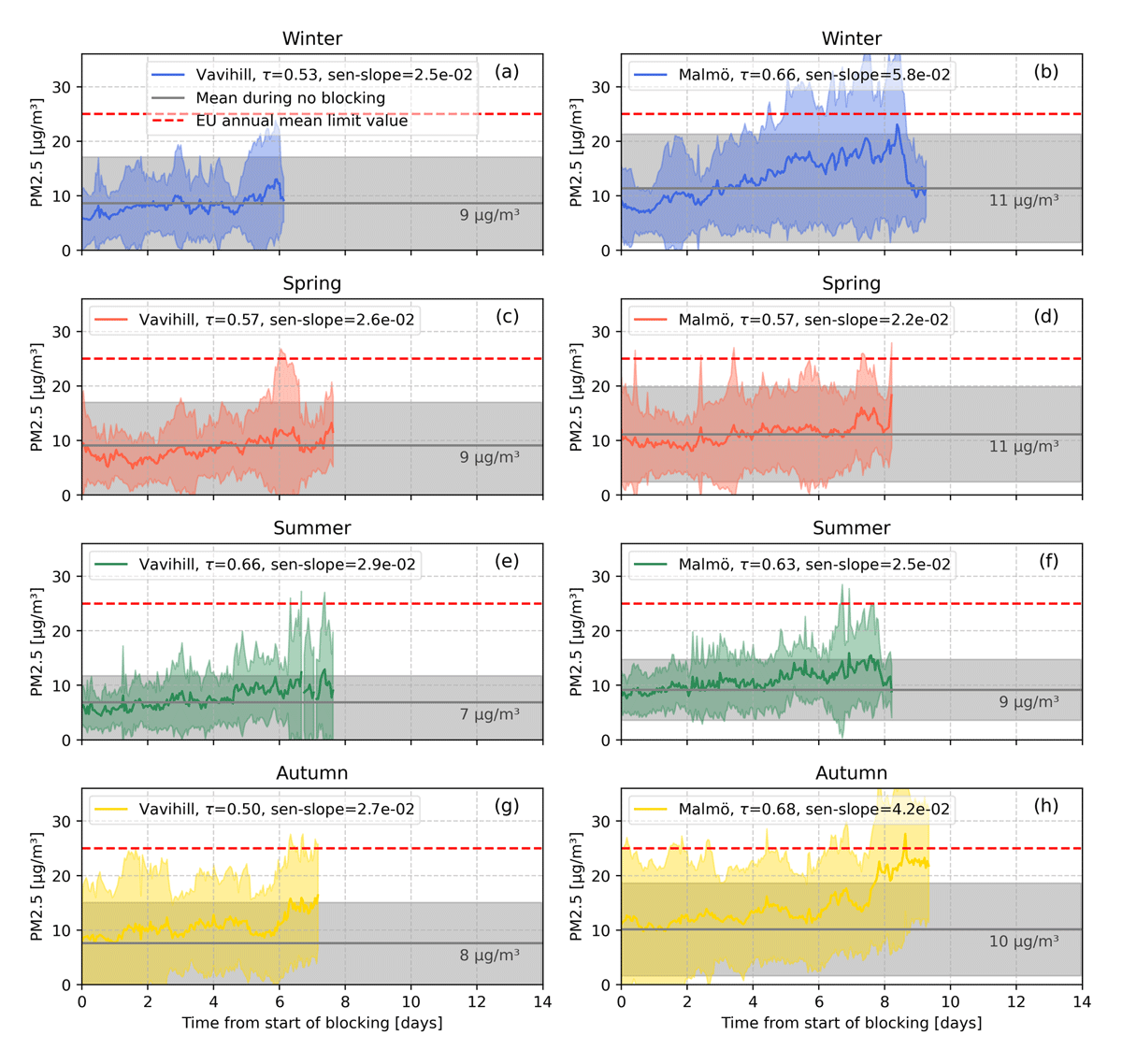
Figure 7

3.1.3 The change in aerosol concentrations depending on high-pressure blocking strength

Lastly, the data was categorised based on the strength of the high-pressure blocking, where a weak high-pressure blocking event had a mean atmospheric pressure between 1014 hPa and 1020 hPa, a medium strong event had a mean atmospheric pressure between 1020 hPa and 1026 hPa, and a stronger event had a mean atmospheric pressure over 1026 hPa. Categorising the events based on pressure provides insight into how the strength of the high-pressure influences the observed aerosol concentration. The categories were chosen based on the clear steps, even separation, and sufficient sample size in each category.

The increase in PM2.5 concentrations depending on the strength of the high-pressure blocking event can be seen in Figure 8. In the case of Vavihill, 22.1% of the blocking events occurred with a mean pressure below 1020 hPa, 53.8% occurred between 1020 and 1026 hPa and 24.0% occurred with a mean pressure over 1026 hPa. In the case of Malmö, 16.1% of the blocking events occurred with a mean pressure below 1020 hPa 59.2% occurred between 1020 and 1026 hPa and 24.7% occurred with a mean pressure over 1026 hPa.

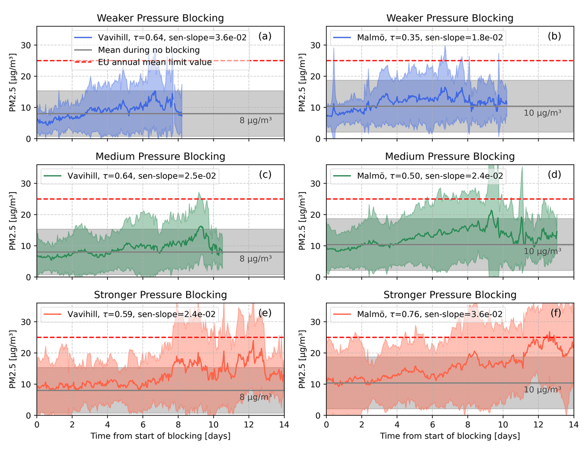
Figure 8

From the plots, one can observe similar behaviour for the two locations. For the weaker high-pressure blocking events there is no prolonged increase, nor highly elevated levels of PM2.5 in either location (Figure 8a & 8b). In the case of medium strong high-pressure blocking events there is a stronger increase in Vavihill τ = 0.64 and a weaker increase in Malmö τ = 0.50. When observing both plots, one can see a maximum around day nine, although the values at maximum PM2.5 levels in Malmö have a larger spread (Figure 8c & 8d). For the stronger high-pressure blocking events one can see a strong increase in the case of Malmö and Vavihill, although the increase in Vavihill is slightly weaker. In Figure 8e & 8f it can be seen that the levels of PM2.5 in Vavihill and Malmö exceed the normal range around day 8 and day 12, where the mean reached the EU annual mean limit value for Malmö. In Vavihill, the values went from 8 µgm^–3 to a maximum of 24 µgm^–3, and in Malmö they went from 12 µgm^–3 to a maximum of 27 µgm^–3.

3.2 The frequency of high-pressure blocking events

The last task of this study was to evaluate whether high-pressure blocking events had become increasingly more common in southern Sweden over the past 75 years. This was evaluated in two different ways: by calculating the number of days under high-pressure blocking events per year, and by the number and lengths of high-pressure blocking events per year. The number of days of blocking was also sorted by the season of the blocking to provide more insight into the nature of the high-pressure blocking events.

When observing the number of high-pressure blocking events per year, no significant change in frequency could be seen (see Figure 9). Since the highest levels of PM2.5 occurred toward the end of the events (see Figures 4, 8), the frequency of longer high-pressure blocking events was also examined. However, no increase could be observed in any of the cases. One must note that the p-values, from the Mann-Kendall test, are much larger here than in Figures 4, 8.

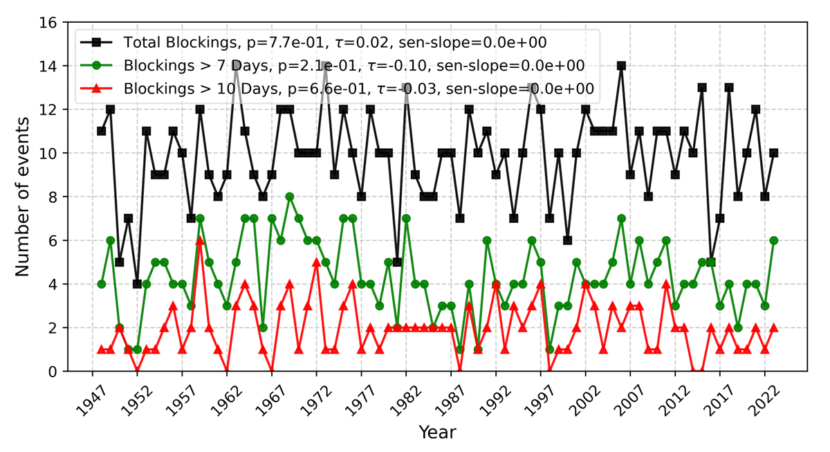
Figure 9

In Figure 10, the number of days with high-pressure blocking events per year can be seen. Similarly to Figure 7, 8 and 9, the blocking events have been divided according to wind direction, season and average pressure during the blocking event. Here, one can observe that the large p-values indicate that there is no statistically significant trend. One can thus observe that no type of high-pressure blocking event has become more common during the last 74 years.

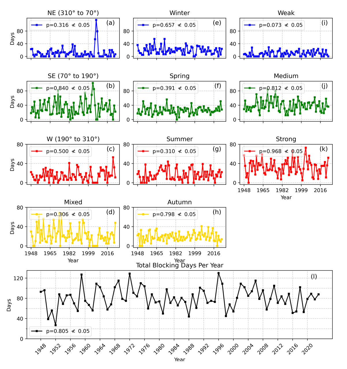
Figure 10

4 Discussion

From Figures 4, 8, a steady increase in PM2.5 during high pressure blocking events can be seen with the highest concentrations of PM2.5 after seven to 13 days into a blocking event. The sudden drops in PM2.5 after day 8 in Figures 4, 8 can be explained by the ending of several high-pressure blocking events with high PM2.5 levels. The accumulative increase of PM2.5 can be seen in Figure 4, where the combination of all the other plots results in a steady increase in the case of Malmö and in Vavihill. Especially strong increases with elevated PM2.5 levels can be seen with winds from the south-east and for stronger pressure high-pressure blocking events.

The European Union mean yearly limit value, 25 µgm^–3, was only exceeded with winds from the south-east and high-pressure blocking events with a mean above 1026 hPa in Malmö. These two categories also yielded elevated levels in Vavihill, although they did not reach the European Union mean limit. One reason why Malmö saw higher aerosol levels could be due to more industrial and traffic activities in Malmö, as well as the city’s closer proximity to central Europe, meaning that the stagnant air during the high-pressure blocking event affected Malmö more. Another argument for why a larger increase was seen in Malmö than in Vavihill could be the difference in ground inversions. Vavihill is located in a rural area with abundant greenery and canopy cover, which would reduce the strength of the inversion, whereas the impervious surfaces in urban Malmö would enhance it. As ground inversion further enhances aerosol levels, this effect would certainly have an impact on the different locations and could help explain the difference in PM2.5 concentrations.

The finding that winds from the south-east increased aerosol levels more than any other direction suggests that long-range advection plays a crucial role in the accumulation of aerosols in the region. The reason why a stronger mean pressure during the blocking events induced a more pronounced aerosol increase could be because these are associated with a stronger high-pressure system and subsidence inversion. However, the difference between advection and local emissions should be further researched, to investigate the main contributor to the rise in aerosol levels.

As aerosol levels have a significant impact on human health, our findings regarding rising PM2.5 levels during high-pressure blockings are relevant for the county of Skåne. The results are particularly relevant for the city of Malmö, which has a large population, as the results demonstrate that air quality in the city worsens during anticyclones. Since anticyclones can be easily monitored in real time, this information could provide a practical tool for authorities in Malmö and across Skåne to prepare for periods of worsening air quality.

This study showcased an increase in PM2.5 during high-pressure blocking events, which agrees with Dempsey (2018), Messori et al. (2018), Shin et al. (2021) and Özdemir, Birinci, and Deniz (2024). Both Messori et al. (2018) and Özdemir, Birinci, and Deniz (2024) predicted that increases are stronger in urban areas, which was observed in this study with the larger increase in Malmö than in Vavihill. The findings in this study also showcased that different wind directions led to different amounts of aerosol increase. The dependence of wind patterns was demonstrated by both Dempsey (2018) and Shin et al. (2021), which this study agrees with. Furthermore, the aerosol increases seen by Grundström et al. (2017) during anticyclones are supported by this study.

We find that no type of high-pressure blocking event had become more frequent during the last 74 years. This opposes the findings from Lupo (2021), who saw an increase in high-pressure blockings during the last 50 years. However, those observations were for the entire Northern Hemisphere. Similarly, Coumou, Lehmann, and Beckmann (2015), suggested that the Northern Hemisphere summer circulation significantly weakened between 1979 and 2013, a change that would be expected to increase the frequency of high-pressure blocking events during summer. Moreover, Francis and Vavrus (2015), found that rapid Arctic warming during 1994 to 2013 in the Northern Hemisphere mid-latitudes, is associated with more persistent weather, such as high-pressure blocking. On the other hand, a European-centred study by Fahimi et al. (2020) showed a decrease in high-pressure blocking events between 1959 to 1988, and an increase from 1989 to 2011. This is more in line with the findings in this study, highlighting temporal variability in the blocking frequency trend. In Figure 9, a small decrease is prominent between 1948 to 1998, which shows that this study does not oppose the findings by Fahimi et al. (2020). Furthermore, the findings in this study align with Blackport and Screen (2020), who showed that although Arctic amplification is occurring, the mid-latitude circulation in the Northern Hemisphere has not become wavier during the period 1979 to 2018. Thus, high-pressure blocking has not increased during this time but instead varies due to natural variability.

5 Conclusion

This study has demonstrated that the presence of high-pressure blocking events in southern Sweden significantly increased the aerosol concentration in both rural and urban locations. The mean PM2.5 in Malmö went from 10 µgm^–3 to a maximum of 22 µgm^–3 during the high-pressure blocking events, and an average increase from 7 µgm^–3 to a maximum of 19 µgm^–3 was observed in Vavihill during the events. High levels of PM2.5 were seen in both locations after seven to 13 days of high-pressure blocking, indicating accumulation of aerosols during the events. This accumulation was mainly attributed to the presence of a subsidence inversion layer, which prohibits vertical air mixing. It was also observed that once the high-pressure blocking event ended, aerosol levels returned to normal within a day. A stronger increase in PM2.5 was found in the urban area of Malmö than the rural area of Vavihill, which was mainly attributed to local emissions and possibly a slightly stronger ground inversion, especially during the winter. The wind directional dependence on PM2.5 concentrations indicated that the long-range advection of aerosols was a significant contributor to aerosol concentration in the region, where winds from central and eastern Europe significantly increased the aerosol levels. The seasonal dependence indicated a stronger increase in PM2.5 levels during blocking events during winter. A stronger increase was also observed with higher average pressure during blocking events, where the highest levels of PM2.5 was observed. The length and number of high-pressure blocking events has not increased during the investigated 74 years, which aligns with other European studies.

The analysis of aerosol concentrations during meteorological events is important for monitoring the health risks associated with different meteorological phenomena. Local authorities in Malmö and the county of Skåne can use the findings of this study to better monitor the negative health effects of meteorological events on the people in the region. This study has shown that it is not only local emissions that play a role in air quality, but that advection from nearby countries also plays a crucial role. This shows the importance of international work to prohibit the large-scale emissions of aerosols. As the climate changes, so does the weather, and understanding how these changes affect us is of utmost importance.

Data Accessibility Statement

The data used in this study has been downloaded from SMHI meteorological archive and the SMHI air concentration portal. The full source code and data files for this study are available on GitHub. The repository includes all Python scripts used for data processing, statistical analysis, and figure generation. Please refer to the ‘README.md’ file in the repository for an overview of the file structure and dependencies. The code is licensed for academic use, and citation of the work is appreciated.

Competing Interests

The authors have no competing interests to declare.

Author Contributions

M. K. S. designed the research idea. F. B. has downloaded all data and performed the data analysis with supervision from M. K. S.. F. B. wrote the manuscript and M. K. S. reviewed and commented on it. The authors have together discussed the findings in the manuscript.