
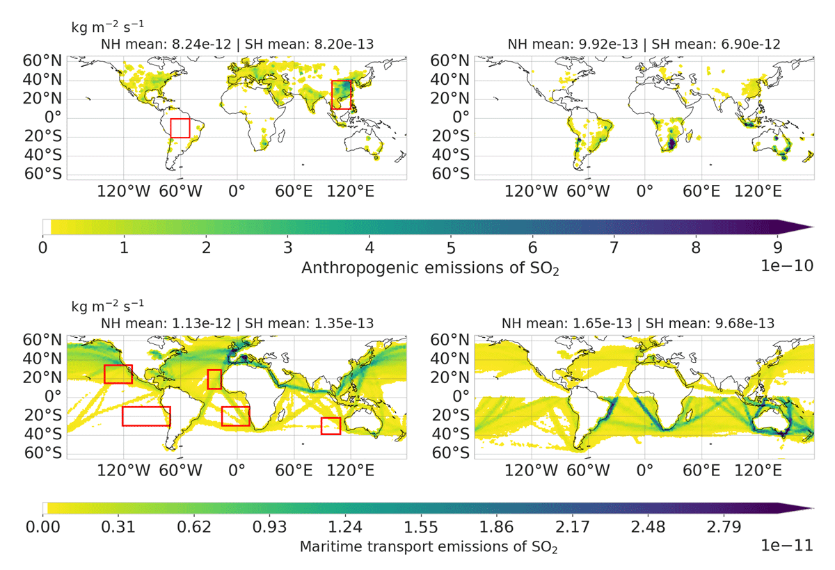
Figure 1
Global distribution of the annual mean (2003–2010) maritime transport emissions of sulfur dioxide (SO2) before flipping emissions (ICON-HAM CTRL, left lower panel) and after flipping emissions (ICON-HAM FLIP, right lower panel) and of the annual mean anthropogenic emissions of (SO2) (total sectors) (ICON-HAM CTRL, left upper panel) and after flipping emissions (ICON-HAM FLIP, right upper panel). The red boxes over regions illustrate the selected regions over land and stratocumulus regions over ocean, which is discussed in Section 3.2.2.
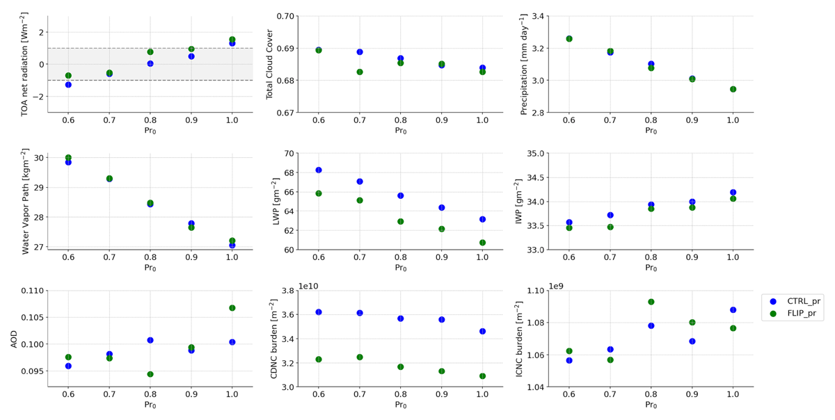
Figure 2
One-year sensitivity simulation to variations in the neutral limit Prandtl (Pr0) number, ranging from 1 to 0.6 CTRL and FLIP configurations. Net radiation TOA, total cloud cover, precipitation, water vapour path, cloud liquid water path (LWP), ice water path (IWP), aerosol optical depth (AOD), cloud droplet number concentration burden (CDNC burden), vertically integrated ice crystal number concentrations as a function of neutral limit Prandtl (Pr0) number. The default value for Pr0 in the CTRL and FLIP simulations is 0.8.
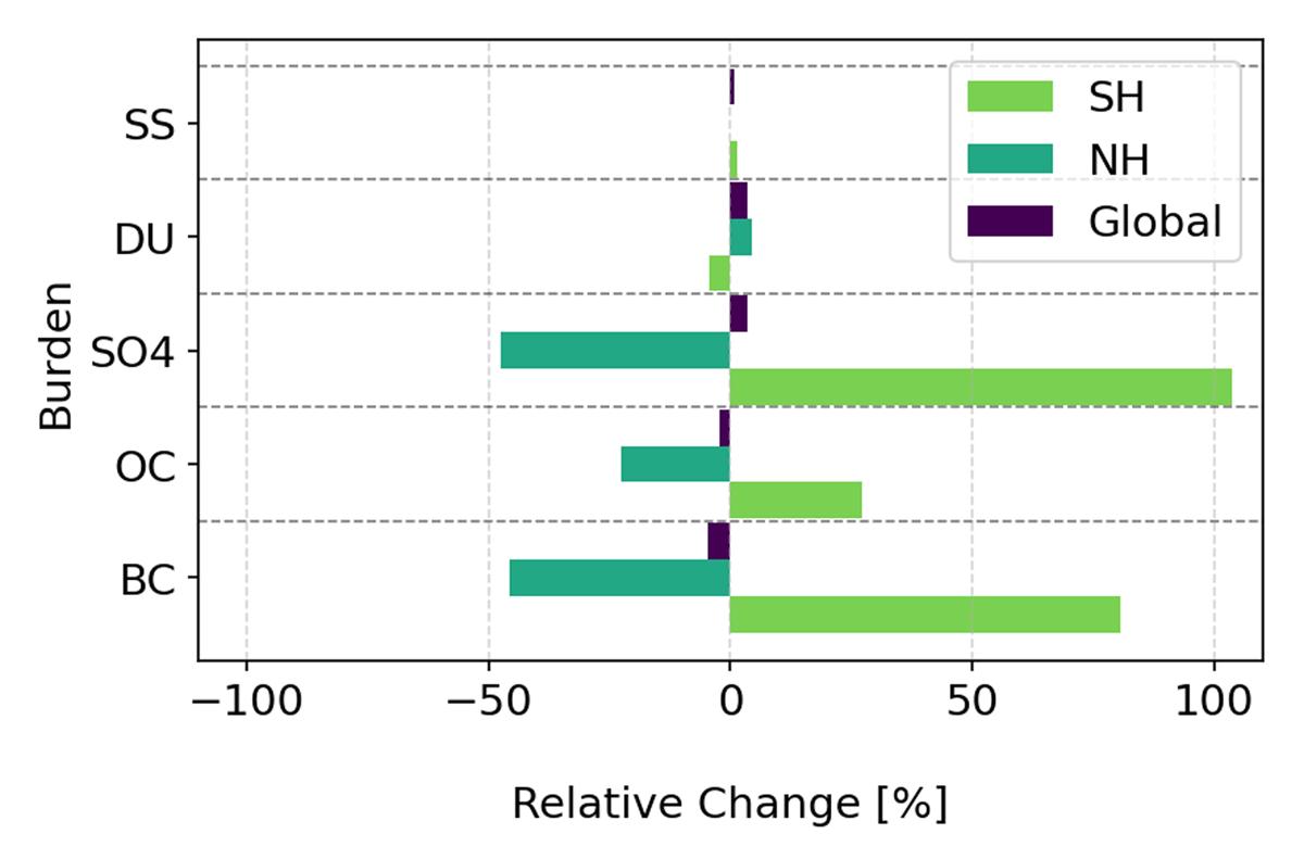
Figure 3
Global and hemispheric atmospheric aerosol burden as relative changes between the FLIP and CTRL simulations . SS, DU, SO4, OC, and BC stand for the major aerosol global compounds, sea salt, mineral dust, sulfur dioxide, organic carbon, and black carbon respectively.
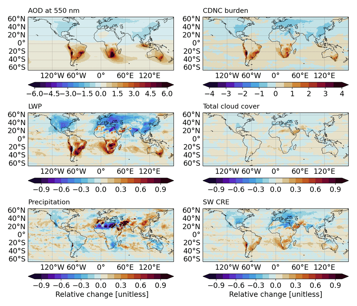
Figure 4
Relative changes in spatial distributions of FLIP simulation in comparison to the CTRL simulation . Direct diagnostics output of the model of aerosol optical thickness total at 550 nm (AOD), cloud droplet number concentration burden (CDNC burden), vertically integrated cloud water (LWP), total cloud cover, precipitation and shortwave cloud radiative effect (SW-CRE).
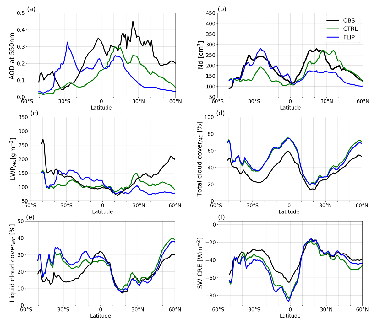
Figure 5
Zonally averaged multi-year means of (a) aerosol optical thickness at 550 nm, (b) cloud droplet number concentration (Nd), (c) liquid water path (LWP), (d) total cloud cover, (e) liquid cloud cover, and (f) shortwave cloud radiative effect (SW-CRE) from the control simulation (CTRL, green line), the flipped anthropogenic aerosol emissions simulation (FLIP, blue line), and observations (OBS, black line; MODIS for aerosols, MODIS COSP dataset for clouds, CERES for radiation).
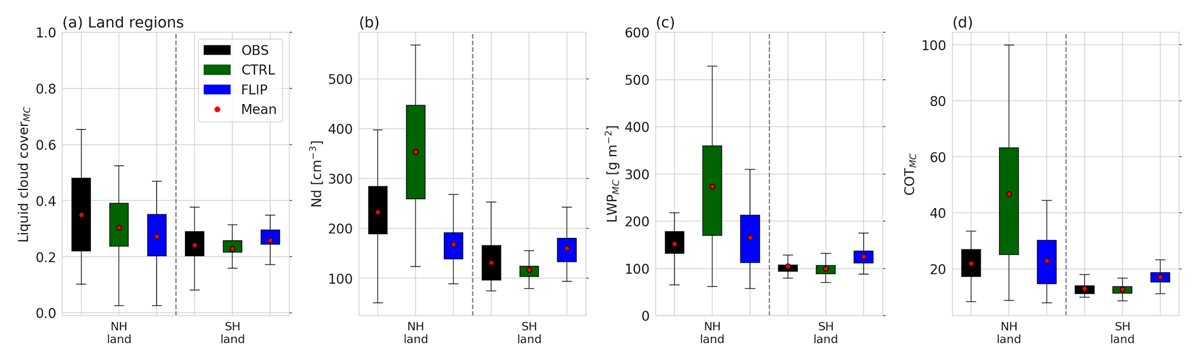
Figure 6
Liquid cloud properties statistics simulated by the MODIS-COSP (MC) in the CTRL and FLIP configurations (green and blue colour, respectively), compared to the observational dataset (black colour). Eight years of annual average boxplots for (a) liquid cloud fractionMC, (b) liquid water path (LWPMC), (c) droplet number concentration (Nd), and (d) cloud optical depth (COTMC), over two contrasting land regions in Southeast Asian (NH land) and Amazonia Rainforest (SH land) as marked in Figure 1.
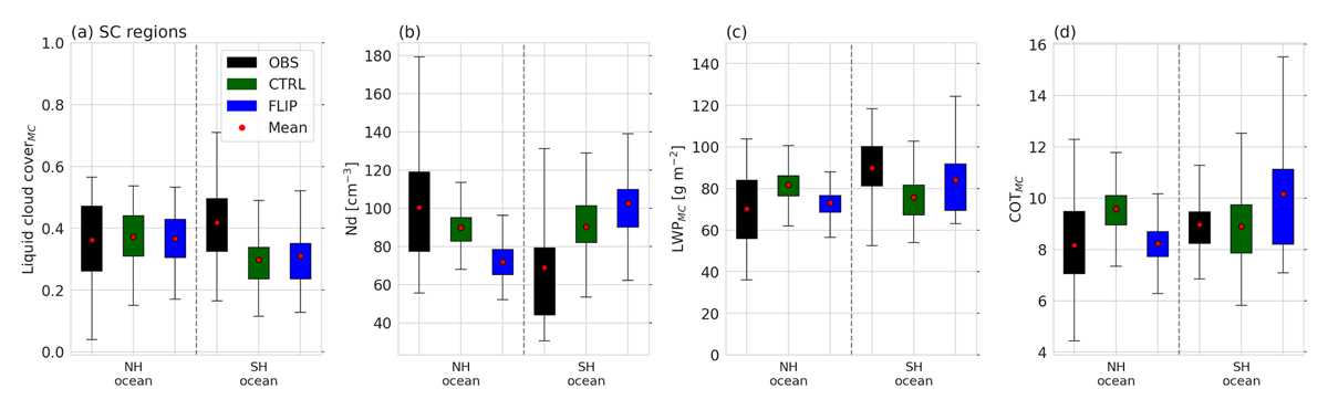
Figure 7
Same as Figure 6 but over marine stratocumulus regions. The black, green, and blue colour boxes correspond to MODIS-COSP observation, and diagnostics from MODIS COPS simulator in CTRL and FLIP simulation, respectively.
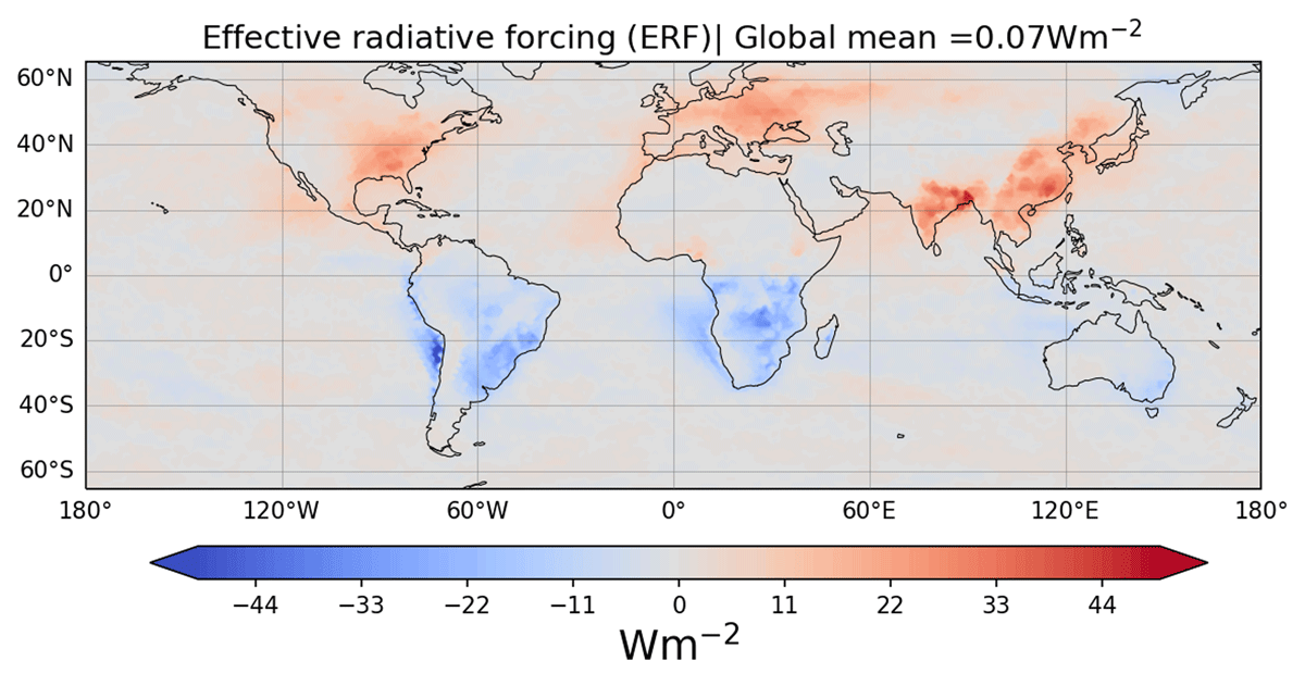
Figure 8
Effective radiative forcing (ERF) from flipping emissions between hemispheres. The ERF was calculated as the difference of the TOA net radiative flux between the FLIP and CTRL simulations.
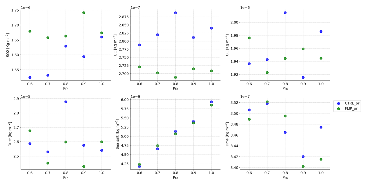
Figure A1
Sensitivity of a one-year simulation of aerosol burdens to variations in the neutral limit Prandtl (Pr0) number, ranging from 1 to 0.6. The default value for Pr0 in both the CTRL and FLIP simulations is 0.8.
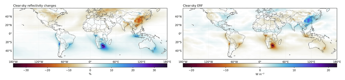
Figure A2
Clear-sky diagnostics between FLIP and CTRL. Left: reflectivity changes (%). Right: clear-sky effective radiative forcing (W m–2).
Table A1
Comparison between the simulations and global observational dataset in terms of cloud properties. Global eight-year annual mean values for key liquid cloud properties using the MODIS COSP simulator in ICON1.3.0-A-HAM2.3 and the MODIS COSP dataset. The OBS used is Nd cloud top (3.7 µm) uses Nd_G18_37 from (Grosvenor and Wood 2018). For the total cloud cover, liquid cloud coverliq, Cloud Effective Radius (CERliq(MC)), Cloud Optical Thickness COTliq, and LWP are from the MODIS COSP (MC) dataset and simulator.
| VARIABLE | OBS | CTRL | FLIP |
|---|---|---|---|
| Nd cloud top (3.7 µm) [cm–3] | 90 | 102 | 98 |
| Total cloud coverMC [%] | 46 | 33.5 | 33.4 |
| Liquid cloud coverMC [%] | 13 | 14.2 | 14.3 |
| CERliq(MC) [µm] | 13.5 | 7.3 | 7.4 |
| COTliq(MC) | 15.3 | 9.2 | 8.8 |
| LWP(MC) [g m–2] | 133.1 | 70.3 | 68.3 |