
1. Introduction
Changes in atmospheric aerosol concentration are bound to affect cloud properties, rain formation rates, and cloud radiative effects (Fan et al. 2016; Bellouin et al. 2020). Aerosols exert an effective radiative forcing (ERF) on climate through their interactions with both radiation and clouds (Boucher et al. 2013). The former occurs through the scattering and absorption of sunlight by aerosol particles, while the latter arises from their role as cloud condensation nuclei, which modify cloud microphysical and radiative properties. The interactions between aerosols and clouds remain the major source of uncertainty in current estimates of the effective radiative forcing attributed to anthropogenic aerosol relative to preindustrial (PI) climate conditions (IPCC 2021). Over the industrial period, anthropogenic aerosol emissions and their precursors have increased primarily in the Northern Hemisphere (NH) compared to the Southern Hemisphere (SH). This has resulted in a distinct feature: the hemispheric contrast in the anthropogenic aerosol forcing. This contrast is closely associated with the short tropospheric lifetime of aerosols, entangled with their effects in the hemispheric scale of the source locations (Schwartz 1988; Feng and Ramanathan 2010; Quaas 2015).
Climate forcing over both the historical era and projected future scenarios involves changes in anthropogenic forcings, such as aerosols and greenhouse gases (Wang et al. 2021), as well as changes in their emission location, distribution, and composition (Lund, Myhre and Samset 2019; Williams et al. 2022). Over the past 20 years, both hemispheres have experienced changes, with varying concentrations and types of anthropogenic atmospheric aerosols in particular locations (Quaas et al. 2022). These trends differ among the major aerosol species: sulfur dioxide (SO2) and organic carbon (OC), which are predominantly scattering and hydrophilic, have generally decreased in the Northern Hemisphere. Absorbing black carbon (BC) has shown more regional variability, with increases over parts of South and Central Africa and South Asia. Such compositional differences determine whether aerosols act mainly as cloud condensation nuclei or as light-absorbing particles, thereby influencing both cloud microphysics and radiative effects. In the NH, emissions trends have seen a decrease over Europe and North America, as well as in parts of Asia, such as China, while in other regions, particularly over India and portions of Africa, trends in anthropogenic aerosol emissions have been increasing (Jia and Quaas 2023). The SH, in turn, has seen less consistent changes. Over South America and Australia, decreases in aerosols are mostly prevalent, while over portions of Africa, aerosol levels increased. For the future, growth in anthropogenic aerosol emissions in the SH is projected in Shared Socioeconomic Pathways future scenarios (Lund, Myhre and Samset 2019).
Exploring how liquid cloud properties will respond to changes in the concentration and spatial distribution of anthropogenic aerosol is an important issue for climate sensitivity in both the present-day and projected future scenarios. Liquid clouds were identified to be the most significant cloud regime resulting in effective radiative forcing due to aerosol-cloud interaction (Bellouin et al. 2020). The main way that anthropogenic aerosols affect liquid clouds is by enhancing the concentration of cloud condensation nuclei and, in turn, increasing the concentration of droplet number, Nd (Twomey 1974). Changes in Nd affect cloud optical characteristics, but in consequence also affect the microphysical processes of clouds, rain formation, and, thus, cloud lifetime (Albrecht 1989). However, the response of cloud liquid water content to the changes in aerosol and Nd is more complex (Gryspeerdt and Stier 2012; Gryspeerdt et al. 2019; Possner et al. 2020; Toll et al. 2019; Grosvenor and Wood 2018) and differs as a function of meteorological conditions or cloud macro properties. The response of cloud cover to anthropogenic aerosol contributes significantly to the uncertainty in effective radiative forcing. While satellite observations provide some constraint (Quaas et al. 2022), global models still disagree even on the sign of the cloud fraction response to aerosol perturbations (Mülmenstädt et al. 2020; Duran et al. 2025), and the influence of aerosols on cloud fraction remains poorly constrained (Bellouin et al. 2020).
Previous studies have addressed the hemispheric contrast in anthropogenic emissions as a global experiment (Schwartz 1988) and its implications for observing anthropogenic aerosol-cloud interactions using global satellite retrievals (Quaas 2015; McCoy et al. 2020; Cao et al. 2023). (McCoy et al. 2020) have shown that the present-day (PD) observed differences in oceanic aerosol perturbation between hemispheres help to obtain clues about aerosol radiative forcing between PD-PI. They observationally constrain aerosol radiative forcing using the satellite Nd(NH–SH), with Nd(SH) in Southern Ocean regions (30°S–60°S) serving as a PI proxy and the Nd(NH) in the polluted Northern Hemisphere Ocean (30°N–60°N) as PD. Along these lines of identifying the impact of changes in anthropogenic aerosol emissions between hemispheres, Cao et al. (2023) found a significant decrease in marine Nd(NH–SH) trends due to a strong decrease in emissions over the NH. From observed NH-SH differences in satellite observations, the hemispheric contrast was also used to evaluate the simulation of cloud properties in global climate models (GCMs) (Boucher and Lohmann 1995; McCoy et al. 2020; Wang et al. 2021).
Other studies have used GCMs to examine how the change in the location of aerosol emission will impact the effective radiative forcing of the climate. Examples of these changes include increased absorbing aerosol (Williams et al. 2022) or decreased fossil fuel emissions and their effects on precipitation and cloud cover, and the resulting impact on the net radiative energy flux into the climate system (Peters et al. 2012; Williams et al. 2022, 2023; Persad 2023). Peters et al. (2012) quantify the aerosol indirect effects of ship emissions and the effect of reducing carbonaceous emissions. Williams et al. (2022) discuss the dependence of absorbing aerosol on effective radiative forcing due to aerosol-radiation interaction and Persad (2023), the influence of the geographic distribution of aerosol emission on precipitation.
As an attempt for detection and attribution, we explore the hemispheric differences in anthropogenic aerosol distributions by conducting a sensitivity experiment using the aerosol–climate model ICON1.3.0-A-HAM2.3 (Salzmann et al. 2022). The ‘flipping emission’ experiment involves varying the major anthropogenic emissions by scaling aerosol levels based on those from the counterpart hemisphere, specifically increasing emissions in the SH and decreasing them in the NH. This setup represents a counterfactual framework designed to quantify the influence of hemispheric contrast in anthropogenic emissions on clouds and radiation. In this hypothetical scenario, the bulk of anthropogenic activities would occur in the SH rather than the NH, while the global total would remain unchanged. This study addresses two key aspects: the impact of changes in aerosol concentration on cloud properties, and the influence of hemispheric emission distribution on radiative forcing.
2. Methodology
2.1 Aerosol-Climate Model ICON-HAM
The icosahedral non-hydrostatic global atmosphere model ICON-A (Giorgetta et al. 2018), version icon-aes-1.3.00, coupled to the Hamburg Aerosol Module (HAM; Stier et al. 2005) Version 2.3 (HAM2.3; Tegen et al. 2019) is used in this study, which is described in Salzmann et al. (2022). The HAM aerosol module is a modal aerosol microphysics parameterisation in which the major aerosol species sulfate, black carbon (BC), organic carbon (OC), sea salt, and mineral dust are assumed to be internally mixed particles in seven different size distribution modes. The aerosol processes are represented by the M7 aerosol microphysics module (Vignati, Wilson and Stier 2004). In M7, the modes are separated into three hydrophobic and four hydrophilic modes of log-normal size distributions, each containing one or more internally-mixed species. Thus, in the ICON1.3.0-A-HAM2.3 Aerosol-Climate Model, the aerosol precursors and aerosols are emitted, transported, transformed, and removed (Salzmann et al. 2022; Tegen et al. 2019). Hereafter, the ICON-A-HAM2.3 Aerosol-Climate Model will be referred to as ICON-HAM.
ICON-HAM has the Max Planck Institute physics package (Stevens et al. 2013; Mauritsen et al. 2019) implemented. The parametrisations of physical processes in ICON-A are described in (Giorgetta et al. 2018). The solar (shortwave) and terrestrial (longwave) radiation is parameterised using the PSrad scheme based on Pincus and Stevens (2013) as a further development of the rapid radiative transfer model optimised for general circulation models (RRTMG; Iacono et al. 2008). Stratiform cloud cover is computed as a function of relative humidity based on (Sundqvist, Berge and Kristjánsson 1989). The two-moment cloud microphysics scheme with prognostic cloud droplet and cloud ice crystal number concentrations is based on (Lohmann and Neubauer 2018) and (Lohmann et al. 2007). The Köhler-theory-based cloud droplet activation scheme follows (Abdul-Razzak and Ghan 2000). Convection is parameterised using a mass-flux scheme (Tiedtke 1989; Nordeng 1994). The vertical diffusion parametrisation is a total turbulent energy scheme (TTE) that is described by Mauritsen et al. (2007) and later modified by Angevine, Jiang and Mauritsen (2010) and Pithan, Angevine and Mauritsen (2015). The land surface model is the JSBACH4 used in a simplified configuration version referred to as ‘JSBACH4-lite’ (Giorgetta et al. 2018).
To compare the simulated liquid cloud properties with satellite observation properly, the Cloud Feedback Model Intercomparison Project (CFMIP) Observation Simulator Package (COSP) (Bodas-Salcedo et al. 2011) version 2.0 (Swales et al. 2018) for cloud retrievals by the MODerate Resolution Imaging Spectroradiometer (MODIS) sensors (Platnick et al. 2017) was implemented into the ICON-HAM model. The simulator combines the features of MODIS instruments and model fields, taking into account the limitations of satellite data and model characteristics (Saponaro et al. 2020; Pincus et al. 2023).
The present study discusses two configurations based on the Atmospheric Model Intercomparison Project (AMIP) setup experiment with prescribed sea surface temperature and sea-ice cover distributions (Taylor et al. 2012). The horizontal resolution used is the triangular R2B4 horizontal grid (Giorgetta et al. 2018), featuring a grid resolution of approximately 160 km in the horizontal and a vertical hybrid sigma height coordinate with 47 vertical levels.
2.2 ‘Flipping emission’ experiment and sensitivity studies
We explore two AMIP configurations conducted with the ICON-HAM. For the control (CTRL) configuration, we used the monthly mean anthropogenic and biomass-burning aerosol and aerosol precursor gas emissions from the AeroCom-II ACCMIP database following the Representative Concentration Pathway (RCP) 8.5 scenario (Van Vuuren et al. 2011) data from 2002 to 2010. In contrast, the other configuration involved flipping anthropogenic emissions between hemispheres. The flipped emission experiment (FLIP) used the reference setup CTRL, but used counterpart hemisphere aerosol levels as the scaling rate. Only the emissions of anthropogenic and biomass burning aerosols were flipped between hemispheres, with relevant sectors including industry, energy, burning of agricultural waste, domestic travel, land transportation, and aviation. The distributions of the CTRL natural aerosol emissions, including volcanic sulfur emission, mineral dust, sea salt, and dimethyl sulfide (DMS), are as described in (Salzmann et al. 2022), and they are not modified for the FLIP configuration.
To modify emissions, we scaled Southern Hemisphere (SH) values based on the mean emissions in the Northern Hemisphere (NH), ensuring proportional scaling across regions. The hemispheric mean values were computed as annual averages and applied uniformly across all time steps. The modified distribution of emissions in the SH, denoted as S′(lat, lon, t), is given by:
This equation indicates that the SH emissions are scaled by the ratio of the mean NH emissions N to the mean SH emissions S, and then multiplied by the original emissions at each location S0.
Similarly, the modified distribution of emissions in the NH, denoted as N′, is defined as:
Here, NH emissions are scaled by the inverse ratio , and applied to the original NH emissions N0 at each location. Figure 1 shows the global distribution of original emissions (left) and the modified, hemispherically flipped distribution (right) for maritime sulfur dioxide (SO2) transport (upper panel) and anthropogenic SO2 emissions over land (lower panel). For instance, flipping the maritime or anthropogenic SO2 emissions between hemispheres leads to localised increases or decreases, especially over regions with pre-existing anthropogenic sources. The same scaling procedure was applied consistently to all major anthropogenic and biomass-burning aerosol components ((SO2), BC, and OC) and their respective emission sectors, such as industry, energy production, transport, and biomass burning.
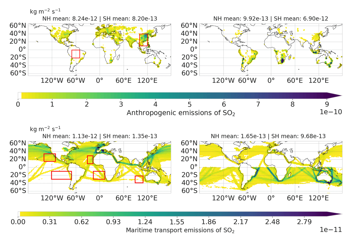
Figure 1
Global distribution of the annual mean (2003–2010) maritime transport emissions of sulfur dioxide (SO2) before flipping emissions (ICON-HAM CTRL, left lower panel) and after flipping emissions (ICON-HAM FLIP, right lower panel) and of the annual mean anthropogenic emissions of (SO2) (total sectors) (ICON-HAM CTRL, left upper panel) and after flipping emissions (ICON-HAM FLIP, right upper panel). The red boxes over regions illustrate the selected regions over land and stratocumulus regions over ocean, which is discussed in Section 3.2.2.
(a) Sensitivity to Prandtl Number in the TTE scheme
GCMs are often tuned by adjusting parameter settings that influence atmospheric processes to achieve radiation balance. Such tuning often focuses on cloud microphysical or convective processes, for example by modifying aspects like rain and snow formation rates or entrainment rates for convective clouds to enhance or reduce their impact on the top-of-the-atmosphere (TOA) energy balance (Lohmann and Ferrachat 2010; Salzmann et al. 2022). Salzmann et al. (2022) focused their radiation-balance tuning on convective and scavenging parameters but did not explicitly assess boundary layer parameters. In ICON-HAM, sub-grid-scale turbulence from the Total Turbulent Energy (TTE) scheme influences both supersaturation and aerosol activation processes (Lohmann et al. 1999) and is directly coupled to the aerosol emissions interface (Salzmann et al. 2022). However, parameters related to the sub-grid-scale vertical velocity can also influence cloud properties and radiative balance. We therefore vary the neutral Prandtl number in the TTE scheme to learn more about its impact on aerosol–cloud interactions.
Here, we investigate the effect of lowering the neutral Prandtl number in a one-year simulation (2003) after a three-month spin-up period. The neutral Prandtl number (Pr0) refers to the ratio of eddy diffusivity for momentum to eddy conductivity for heat, and it is used as a tuning parameter in the TTE scheme in ICON-HAM. Pithan, Angevine and Mauritsen (2015) demonstrated that reducing Pr0 from 1 to 0.8 in the ECHAM6-TTE atmospheric model resulted in increased warming and humidity in the lower troposphere, along with a reduction in radiation bias within stratocumulus regions. Giorgetta et al. (2018) and Salzmann et al. (2022), however, assumed Pr0 = 1 as the default value in the ICON-A and ICON-HAM models, respectively. As a result, the choice of Pr0 can affect aerosol and cloud interactions. The impact of Pr0 on aerosol- and cloud-related processes, such as cloud–aerosol interactions, is seen in aerosol optical depth (AOD), cloud droplet number concentration (CDNC) burden, and vertically integrated ice crystal number burden (ICNC).
Using the CTRL and FLIP configurations, the sensitivity of net radiation at the TOA, aerosol, and cloud properties in the model diagnostics to varying Pr0 from 1 to 0.6 is shown in Figure 2. Lowering Pr0 from 1 to 0.6 leads to a radiation imbalance of about –1 W m–2. The TOA net radiation is balanced when choosing Pr0 values of about 0.8 to 0.9, remaining within ± 1 W m–2 (Lohmann and Ferrachat 2010). The total cloud cover slightly increases when reducing Pr0 from 1.0 to 0.6. When comparing global annual means of precipitation, water vapour path, and cloud liquid water path (LWP), we observe an increase in the global mean values as Pr0 decreases. In contrast, the ice water path (IWP) gradually decreases from 34 g m–2 at Pr0 = 1 to 33.5 g m–2 at Pr0 = 0.6, indicating a slight impact on the cloud phase with decreasing Pr0 (an increase in LWP as IWP decreases). Reducing Pr0 also leads to changes in aerosol and cloud properties. We observe a decrease in global mean AOD, driven by reductions in aerosol burdens (Figure A1). The slight non-linear increase at Pr0 = 0.8 is linked mainly to enhanced dust, but also to BC and OC burdens (Figure A1), which contribute to AOD in regions less relevant for cloud activation Although the variations are small, the CDNC burden shows a slight increase with decreasing Pr0, while the ICNC burden exhibits a slight decrease as Pr0 is reduced from 1.0 to 0.6.
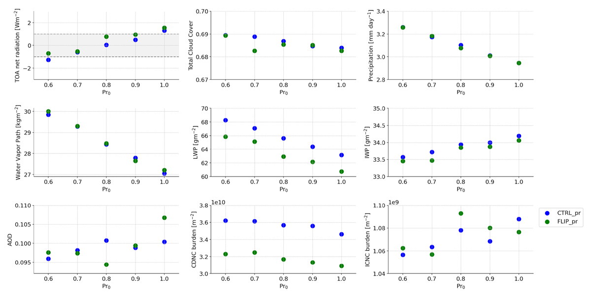
Figure 2
One-year sensitivity simulation to variations in the neutral limit Prandtl (Pr0) number, ranging from 1 to 0.6 CTRL and FLIP configurations. Net radiation TOA, total cloud cover, precipitation, water vapour path, cloud liquid water path (LWP), ice water path (IWP), aerosol optical depth (AOD), cloud droplet number concentration burden (CDNC burden), vertically integrated ice crystal number concentrations as a function of neutral limit Prandtl (Pr0) number. The default value for Pr0 in the CTRL and FLIP simulations is 0.8.
Reducing Pr0 to 0.8 in ICON-HAM increases the total cloud cover while remaining within the TOA net radiation balance range of ± 1 W m–2. Although this alters the model from the unity Pr0 default, it increases global vapour path values compared with ERA-Interim analyses, as described by (Giorgetta et al. 2018). This suggests that Pr0 could serve as a simple proxy for aspects of a warmer and more humid climate state; however, our results indicate that, within the range tested here, the impacts of changing aerosol concentrations and emission locations remain largely insensitive to variations in Pr0, implying robustness of the flipping experiment findings with respect to moderate changes in climate conditions. We have therefore set Pr0 = 0.8, following Pithan, Angevine and Mauritsen (2015), as the default value for both the CTRL and FLIP configurations. The simulations were run for eight years (2003–2010) after a three-month spin-up period.
(b) 2.3 Global observation data
The following observational datasets are used for comparison with the simulations. AOD at 550 nm is obtained from the gridded Level-3 MODerate Resolution Imaging Spectroradiometer (MODIS) sensors aboard the Terra and Aqua satellites (Levy et al. 2013). For radiation, we rely on the Clouds and the Earth’s Radiant Energy System (CERES) Energy Balanced and Filled (EBAF) dataset (Loeb et al. 2018), and for global precipitation, on daily estimates from the Global Precipitation Climatology Project (GPCP) (Adler et al. 2003). For the analysis of cloud properties diagnosed in ICON-HAM using the MODIS COSP simulator, we use the cloud optical properties from the MODIS COSP Level-3 dataset (MCD06COSP; Pincus et al. 2023), which provides 3.7 µm retrievals from both MODIS instruments (Platnick et al. 2017). From this dataset, the liquid cloud effective radius (re) and cloud optical depth (τ) are used to compute the cloud-top droplet number concentration (Nd) following Quaas, Boucher and Lohmann (2006), Nd = α τ0.5re–2.5 with α = 1.37 × 10⁻⁵ m–0.5. The observational reference for Nd is the daily 1° × 1° MODIS dataset from Grosvenor and Wood (2018). To ensure consistency, ICON-HAM Nd was computed for each model grid cell using the same formulation and filtered for liquid-phase clouds (4 < τ < 70, 4 μm < re < 30 μm), where the retrieval is the most reliable (Quaas, Boucher and Lohmann 2006). All global observational datasets are provided at 1° × 1°. To enable comparison, model outputs are extrapolated onto the same regular 1° × 1° latitude–longitude grid.
3. Results and discussion
3.1 Assessing the impacts of changes in anthropogenic aerosol distribution
Figure 3 shows the global and hemispheric atmospheric relative changes in aerosol burdens for the FLIP simulation compared with CTRL. For the major anthropogenic aerosol contributors (SO4, BC), the increases in the SH resulting from the flipping are substantially larger than the decreased values over NH. The increase in SO4 is twice as large as the decrease over NH, with positive relative changes in the SH exceeding 100%, while the SO4 burden is reduced by 47% over the NH. Feedbacks of the aerosol life cycle result in an increase in the global SO4 burden by 5% in the FLIP configuration. For the BC burden, there is an increase of about 80% in the SH and a decrease by 45% in the NH, resulting in a global relative change of –4%. Meanwhile, the changes (decrease and increase) in OC are of comparable magnitude between hemispheres. There is an increase by 27% in the SH, a decrease by 22% in the NH, and a resulting –1.1% global relative change. We note that scaling the distribution of the anthropogenic and biomass burning aerosols also impacts the mineral dust burden. The mineral dust burden (DU) relative changes in the SH, NH, and globally are about –4%, 5%, and 4%, respectively. The reduction in soluble aerosols in the NH weakens the wet scavenging of DU because DU has less chance to be mixed with SO4/OC aerosols. No strong changes are simulated in the sea salt (SS) atmospheric burdens.
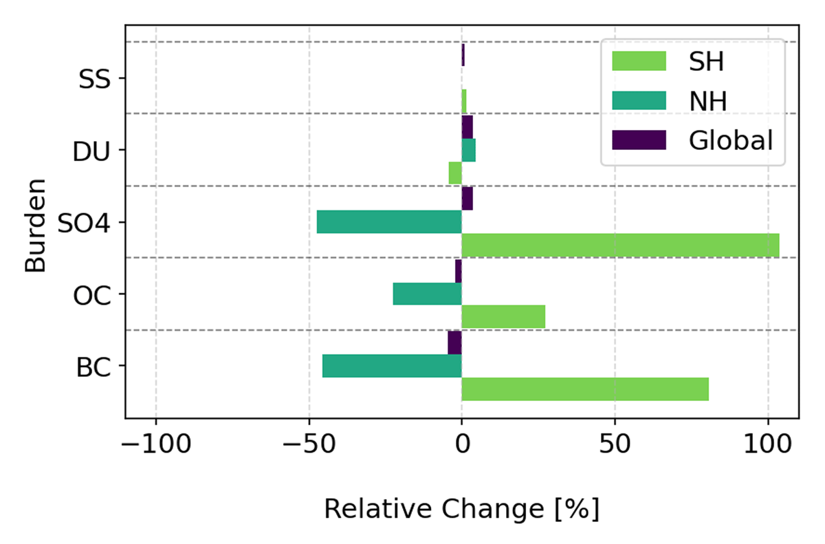
Figure 3
Global and hemispheric atmospheric aerosol burden as relative changes between the FLIP and CTRL simulations . SS, DU, SO4, OC, and BC stand for the major aerosol global compounds, sea salt, mineral dust, sulfur dioxide, organic carbon, and black carbon respectively.
Figure 4 shows the global distribution of eight-year average relative changes in aerosol, cloud properties, and cloud radiative effects from the FLIP simulation compared with the CTRL simulation. The discussion focuses on the region between 60°S and 60°N and on direct diagnostic outputs of the simulation. As expected, the effects of altering the hemispheric contrast in anthropogenic aerosol emissions are evident in AOD, with a clear NH-SH contrast in the global distribution of relative changes. Maximum positive AOD values are seen as the largest positive relative changes in the SH over the continents of South America and Southeast Africa, as well as downwind of these regions. The negative AOD relative changes are observed over the NH with large values across Europe, Asia (largely associated with changes over India and China), and parts of North America. These changes are attributed to the changes in anthropogenic emissions at the source locations. Relative changes in CDNC burden are consistent with the largest changes in AOD over continental regions. Over the SH, the CDNC burden shows significant changes over land and in stratocumulus regions such as the Southeast Pacific and Southeast Atlantic. Over NH midlatitude continents, the negative relative changes come from the same as the negative values of AOD relative changes.
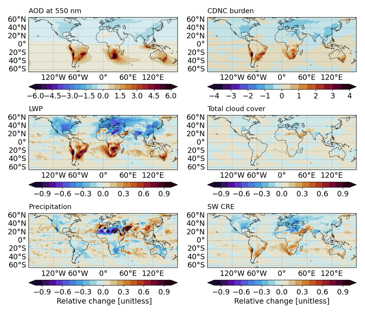
Figure 4
Relative changes in spatial distributions of FLIP simulation in comparison to the CTRL simulation . Direct diagnostics output of the model of aerosol optical thickness total at 550 nm (AOD), cloud droplet number concentration burden (CDNC burden), vertically integrated cloud water (LWP), total cloud cover, precipitation and shortwave cloud radiative effect (SW-CRE).
Changes in CDNC lead to cloud adjustments, the response of cloud horizontal coverage, and the amount of water in the cloud column to CDNC changes (Bellouin et al. 2020; Quaas et al. 2024). In the simulation, LWP and total cloud cover responses vary regionally. Pronounced relative changes in LWP are simulated over the continents and adjacent oceans, with an increase in the SH and a decrease in the NH. A combined analysis of observations and model simulations may help to constrain the magnitude of the effective radiative forcing due to aerosol-cloud interactions. Cloud fraction in the simulation is systematically decreasing over NH continents. This response aligns with regions of reduced CDNC burden and aerosol load. In contrast, over the SH, increased emissions lead to localised increases in total cloud cover, although these are less pronounced compared with the microphysical responses.
The increase in CDNC enhances cloud reflectivity through the Twomey effect, and associated adjustments in cloud fraction and liquid water path lead to more reflective clouds in the SH. The shortwave cloud radiative effect (SW-CRE) therefore shows positive changes in the SH and negative in most parts of the NH, meaning that SW-CRE becomes more negative (stronger cooling) in the SH and less negative in the NH in FLIP compared with CTRL. Reducing anthropogenic aerosols in the NH induces a positive relative change in precipitation, most visible over parts of East Asia, whereas in the SH, increased emissions suppress precipitation over land regions of South America and southern Africa. The simulated precipitation response is non-local and may reflect meteorological variability and large-scale adjustments in circulation and moisture transport, rather than a purely local microphysical effect, consistent with previous studies reporting remote precipitation and circulation responses to regional aerosol perturbations (Westervelt et al. 2020; Persad 2023; Williams et al. 2022; Peters et al. 2012). We also note that large relative changes over NH desert regions arise from very small baseline precipitation and are not physically significant.
To complement the analysis of direct model outputs, we examine key liquid cloud properties of MODIS-COSP-derived quantities in Table A1, which presents global annual mean values from the CTRL and FLIP simulations compared with the MODIS-COSP dataset. The FLIP configuration exhibits a lower global mean cloud-top Nd than CTRL (98 vs. 102 cm–3), while the observed value is even lower at 90 cm–3. Here, the subscript ‘MC’ denotes quantities derived from the MODIS-COSP simulator. Total cloud cover remains nearly identical between the simulations, with CTRL slightly higher than FLIP (∼33.5% vs. ∼33.4%) and notably lower than the MODIS-COSP estimate (46%). In contrast, liquid cloud cover is higher in both simulations than observed in MODIS-COSP and slightly higher in FLIP than CTRL. The other liquid cloud properties, Cloud Effective Radius (CER), Cloud Optical Thickness (COT), and LWP, also show lower global mean values in both FLIP and CTRL compared with the MODIS-COSP dataset: CER is 13.5 μm in observations (OBS) versus 7.4 μm (FLIP) and 7.3 μm (CTRL); COT is 15.3 versus 8.8 and 9.2; and LWP is 133 g m–2 versus 68 g m–2 and 70 g m–2, with FLIP yielding slightly lower COT and LWP than CTRL. A closer look at the response of liquid cloud properties over specific land and ocean geographical locations is presented in Section 3.3, and the impact of cloud property sensitivity on effective radiative forcing is discussed in Section 3.4.
3.2 Zonal mean response over land
The response to changes in anthropogenic aerosol in CDNC and LWP is particularly strong over continents, where most anthropogenic sources are located. To explore the signal of differences, we compare the CTRL simulation and reference observations, not to assess model performance or identify biases in ICON-HAM, but to investigate the model’s sensitivity to aerosol emission changes. Figure 5 shows zonal, temporal averages over land for the CTRL and FLIP simulations compared to OBS. Cloud properties are derived from the MODIS COSP simulator. NdMC are calculated from re and τ and compared with derived MODIS Nd from Grosvenor and Wood (2018). Aerosol and radiation variables are direct model outputs compared to combined Terra–Aqua MODIS and CERES observations.
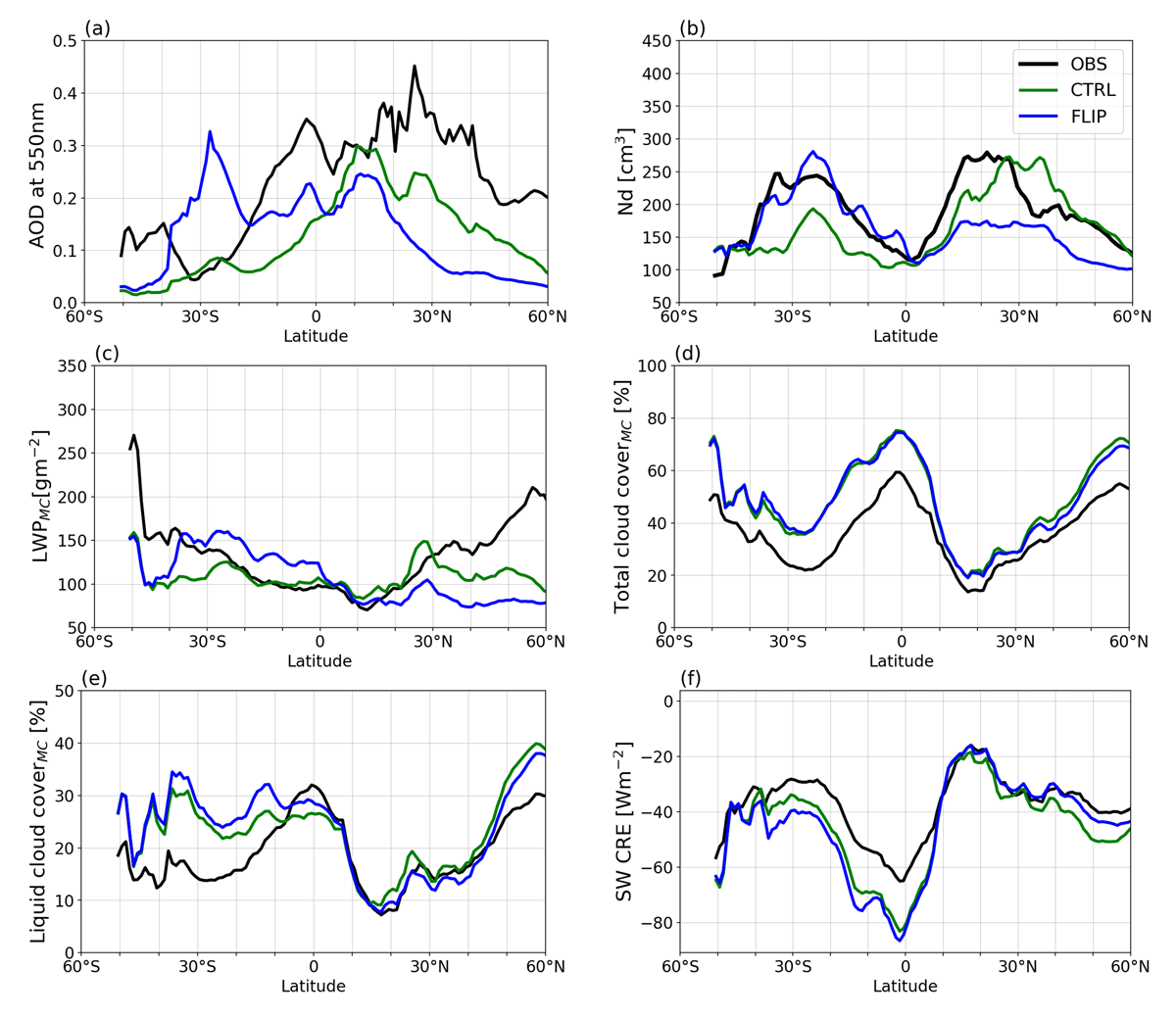
Figure 5
Zonally averaged multi-year means of (a) aerosol optical thickness at 550 nm, (b) cloud droplet number concentration (Nd), (c) liquid water path (LWP), (d) total cloud cover, (e) liquid cloud cover, and (f) shortwave cloud radiative effect (SW-CRE) from the control simulation (CTRL, green line), the flipped anthropogenic aerosol emissions simulation (FLIP, blue line), and observations (OBS, black line; MODIS for aerosols, MODIS COSP dataset for clouds, CERES for radiation).
MODIS AOD (OBS, black lines) show higher values in the NH compared with the SH, as expected. The CTRL simulation (green lines) reproduces the zones of the maximum AOD values, as a result of higher emissions in the NH, but it generally underestimates the values from MODIS retrievals. In the SH, the CTRL simulation only agrees with MODIS AOD around the 30°S, where both CTRL and MODIS AOD show lower values. This negative bias in AOD of ICON-HAM has been highlighted and explored by Salzmann et al. (2022), which described that these differences may be very sensitive to parameter settings in the aerosol module and physics parameterisations. The FLIP simulation (blue lines) clearly shows a hemispheric shift in AOD in which the peak of the maximum values is located in the 20 to 30°S latitude zones, as discussed in the global distribution (Figure 4). In the FLIP NH, the maximum values are located at 10–15°N, and AOD rapidly decreases from 30°N to 60°N.
The OBS Nd (Grosvenor and Wood 2018) shows higher values in the NH than in the SH. Within 20 to 40°S and 10 to 30°N the average values reach the maximum values, with ranges from 200 to 250 cm–3 in the SH and 200 to 275 cm–3 in the NH. The zonal distribution of CTRL NdMC frequently underestimates the OBS Nd, with larger differences in SH. In part of the NH, from 30 to 40°N where the OBS Nd decrease, the CTRL NdMC overestimate the OBS Nd values (Figure 5b). When analysing the FLIP Nd zonal mean, it should be noted that although overestimated, the values from the equator to latitude 30°S in the FLIP agree with the general trends of OBS Nd while the CTRL presents a general underestimation. As mentioned above, when we flipped the emissions, we scaled not only the anthropogenic but also biomass burning emissions. Scaling biomass burning by a factor of 2 or more is known to improve the simulation of AOD in regions impacted or dominated by biomass burning emissions, as is the case of part of the SH (Johnson et al. 2016). It was shown that the increase in biomass burning in the SH improves the Nd values over land but conversely, does not improve the AOD values.
The zonal distribution of observed and CTRL LWPMC shows that the largest differences are located in the extratropical zones in both hemispheres while in SH subtropical and NH tropical land, regions are more comparable. Over the latitude zone from the equator to 40°S, the increase of LWPMC by anthropogenic aerosol in FLIP simulation is seen as a constant overestimation of both CTRL and OBS LWPMC values. Within the NH from 10 to 40°N, the LWPMC FLIP simulation shows a pronounced lower value than CTRL and OBS.
Changing the anthropogenic emissions in the FLIP experiment strongly shifts peaks between extratropic regions, showing higher values between 20 and 30°S and lower between 20 and 30°N in the FLIP compared to CTRL in AOD, Nd, and LWPMC. However, it is interesting to note the modest changes in the zonal distribution differences in total cloud fraction, and liquid cloud cover, in the FLIP and CTRL (Figure 5d-f). CTRL and FLIP underestimate cloud fraction in the extratropical zones, largely in the SH, compared to MODIS COSP data. The liquid cloud cover in the SH FLIP simulation exhibits a slight increase, while the NH exhibits a decrease. The response of SW-CRE is consistent with the response to changes in aerosol in liquid cloud properties. The FLIP simulation shows more negative values in the 20–30°S latitude range, consistent with enhanced microphysical (e.g., Nd, LWP) and, to a lesser extent, macrophysical (cloud fraction) cloud properties. Conversely, their reduction in the NH (10–40°N) under FLIP leads to a weaker SW-CRE compared with CTRL.
3.3 Regional liquid cloud response to flipping emissions between hemispheres
Exploring how liquid cloud properties will respond to changes in the concentration and spatial distribution of anthropogenic aerosol is an important issue for climate sensitivity in both the present day and projected future scenarios. To examine the regional response of cloud properties to changes in aerosol distribution, we focus on contrasting regions with different environments over land and ocean. The locations of the regions are illustrated in Figure 1. Over land in the SH, we show a region of the Amazon rainforest in South America (Herbert and Stier 2023). The Amazon rainforest experiences clean conditions during the wet season and highly polluted conditions with climatologically higher AOD during the dry season (Pöhlker et al. 2018). In contrast, for the NH, we examine parts of the Southeast Asian continent, where satellite observations from 2003 to 2010 showed ongoing growth in anthropogenic aerosol emissions (Quaas et al. 2022). The marine stratocumulus (Sc) regions over the NH and SH are used to illustrate the effects over the ocean. Moderately clean natural conditions are common in the Southern Ocean, whereas Sc regions are often influenced by pollution from ship emissions (Hamilton et al. 2014).
For the major anthropogenic atmospheric burdens in the selected land regions, we find changes similar to those at the hemispheric scale for SO4, BC, and OC (Figure 3). However, the DU burden shows an increase of 50% in Southeast Asia. Figure 6 shows the boxplots of key quantities of MC (MODIS COSP derived parameters) from satellite observations (OBS, black boxes), the CTRL simulation (green boxes), and the FLIP simulation (blue boxes) for Southeast Asia (NH land) and Amazon Rainforest (SH land) regions. The differences in liquid cloud cover between CTRL and FLIP are small, with only a modest increase in the SH and a slight decrease in the NH. When accounting for the portion of liquid clouds not obscured by ice, the results show a small but noticeable increase in liquid cloud cover (not shown), indicating that ice-cloud masking contributes modestly to the apparent differences over land. The decrease in anthropogenic aerosol over Southeast Asia results in a substantial reduction in Nd, from 354 to 168 cm–3 (–52.5% relative change), in LWPMC, from 274 to 166 g m–2 (–39%), and in COTMC, from 47 to 23 (–51.1%). After the flipping, some magnitudes over NH land are comparable with OBS MC. In contrast, the increase in particles over the Amazon Rainforest leads to enhanced mean cloud coverage, with NdMC increasing from 117 to 160 cm–3 (+36.8%), LWPMC from 100 to 125 g m–2 (+25.5%), and COTMC from 13 to 17 (+34.0%). All percentage values refer to relative changes of FLIP with respect to the CTRL simulation. The changes in cloud properties are generally smaller over the Amazon Rainforest compared with Southeast Asia. This result is mainly because of the larger values of Nd and COTMC in Southeast Asia produced by ICON-HAM.
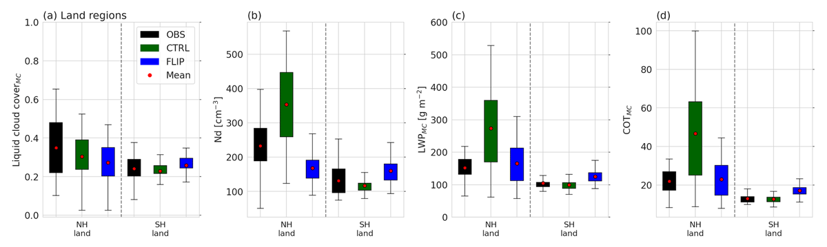
Figure 6
Liquid cloud properties statistics simulated by the MODIS-COSP (MC) in the CTRL and FLIP configurations (green and blue colour, respectively), compared to the observational dataset (black colour). Eight years of annual average boxplots for (a) liquid cloud fractionMC, (b) liquid water path (LWPMC), (c) droplet number concentration (Nd), and (d) cloud optical depth (COTMC), over two contrasting land regions in Southeast Asian (NH land) and Amazonia Rainforest (SH land) as marked in Figure 1.
The changes in aerosol burden over Sc regions are mainly driven by changes in SO4 and BC. Figure 7 shows contrasting NH–SH Sc ocean regions. Unlike over land areas, the simulations of liquid cloud cover show only a slight increase in the SH, from a mean value of 0.317 to 0.331 (+4.4%), and a decrease in the NH, from 0.335 to 0.330 (–1.5%), between the CTRL and FLIP simulations. Over ocean, the difference between liquid cloud cover MC and the non-obscured fraction is small, indicating that the bias there is not primarily caused by obscuration but rather by the simulated amount of liquid cloud itself. Since stratiform cloud fraction in ICON-HAM is diagnosed from relative humidity and not directly linked to aerosols or Nd, changes in microphysical process rates affect it only indirectly. One physical interpretation for the limited change in cloud cover is related to the efficiency of the autoconversion of cloud droplets to rain. When autoconversion remains efficient, aerosol-induced changes in droplet number concentration may not translate into large changes in simulated cloud macrophysical properties such as cloud fraction. Despite the small variations in cloud fraction, there are pronounced changes in microphysical properties. In the NH Sc region, the reduction in anthropogenic emissions leads to a decrease in mean Nd,MC from 110 cm–3 to 88 cm–3 (–20%), in LWP from 72 g m–2 to 64 g m–2 (–11%), and in COT from 9.3 to 8.0 (–14%). Conversely, in the SH Sc region, increasing emissions cause mean Nd,MC to increase from 78 cm–3 to 89 cm–3 (+14%), LWP to increase from 63 g m–2 to 70 g m–2 (+11%), and COT to thicken from 7.0 to 8.0 (+14%).
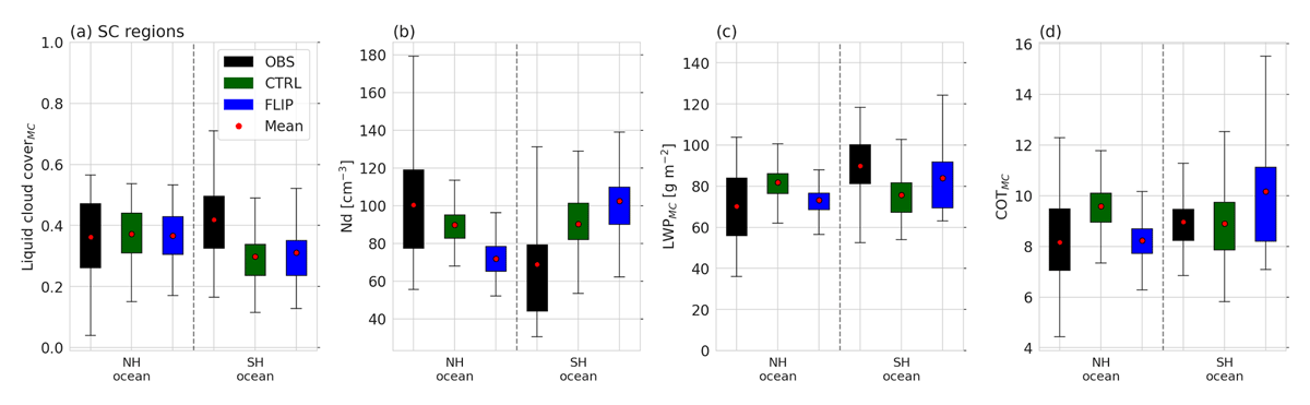
Figure 7
Same as Figure 6 but over marine stratocumulus regions. The black, green, and blue colour boxes correspond to MODIS-COSP observation, and diagnostics from MODIS COPS simulator in CTRL and FLIP simulation, respectively.
3.4 Effective radiative forcing from flipping emissions between hemispheres
Previous studies have linked ERF to emission perturbations, demonstrating that localised reductions could significantly alter radiative forcing and highlighting the sensitivity of climate responses to regional aerosol emissions (Westervelt et al. 2020; Quaas et al. 2022; Persad 2023). The ERF, defined as TOA radiative perturbation due to changes in the emissions distribution, was calculated as the difference in TOA net radiative flux between the FLIP and CTRL configurations. The spatial pattern of ERF is shown in Figure 8. The impact of the reduction of anthropogenic emissions in the NH led to a positive ERF of 2.85 W m–2, consistent qualitatively with the findings by Hodnebrog et al. (2024) and Jia and Quaas (2023), which show that the observed reduction of anthropogenic emissions since 2020 has led to positive ERF values at both regional and global scales. In the SH, the increase in anthropogenic emissions resulted in a negative ERF of 2.63 W m–2 due to increased cloud condensation nuclei concentrations that enhance cloud reflectivity. Our experiment emphasises the impact of anthropogenic aerosol hemispheric distribution of aerosol-cloud interaction in modulating ERF. Positive ERF values over the NH indicate a less negative TOA flux in FLIP than in CTRL, while negative ERF values over the SH indicate a more negative flux in FLIP than in CTRL. Notably, the reduction of the major anthropogenic aerosol emissions in the NH, although smaller than the increase in the SH, contributes more to the global ERF, resulting in a global mean ERF of 0.07 W m–2.
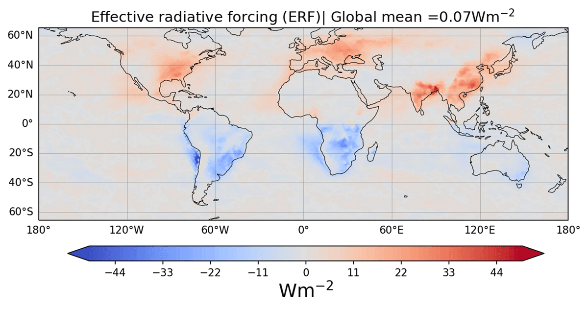
Figure 8
Effective radiative forcing (ERF) from flipping emissions between hemispheres. The ERF was calculated as the difference of the TOA net radiative flux between the FLIP and CTRL simulations.
Variations in ERF between hemispheres are associated not only with changes in cloud properties and cloud adjustments (Figure 4), but also with clear-sky radiative effects (Figure A2). The clear-sky contribution to ERF, calculated as the difference between clear-sky TOA net flux between FLIP and CTRL, amounts to +0.44 W m–2 in the NH, –0.96 W m–2 in the SH. Clear-sky ERF shown in Figure 10 illustrate that aerosol–radiation interactions contribute regionally to the total ERF, with a negative global mean (W m–2), indicating that the overall ERF response is dominated by cloud properties and cloud adjustments. Overall, the NH ERF response is well explained by land-ocean distribution, thicker clouds, and the higher concentration of emissions over densely populated and industrialised regions compared with the SH, which is mostly dominated by oceans. Over Sc regions in the SH, the increase in anthropogenic emissions results in enhanced aerosol-induced cloud brightening, contributing to a localised negative ERF. Marine Sc clouds are frequently studied in the context of marine cloud brightening, a climate intervention strategy involving the injection of particles generated by ocean-based sprayers to offset greenhouse warming (Wood 2021). The SH has a large potential for marine cloud brightening as it is relatively clean and most sensitive to aerosol perturbations. With the increase in anthropogenic aerosol pollution, the flipping experiment, driven mainly by SO4 and BC with relative changes of 100% and 80%, respectively, and a resulting perturbation in Nd of 14%, yields a regional ERF of about –4.47 W m–2 over SH stratocumulus regions. When translated into a global mean equivalent based on the fraction of grid points these regions represent, this corresponds to a global mean ERF of approximately –0.14 W m–2.
4. Conclusion
This study attempts to use changes in the distribution of anthropogenic aerosol emissions between hemispheres as a detection and attribution approach. Using the aerosol–climate model ICON1.3.0-A-HAM2.3, the anthropogenic and biomass-burning aerosol emissions were flipped by hemispheric scaling of the emission source locations. By flipping the aerosol emission distributions between hemispheres, we aimed to isolate the impacts of these spatial differences on cloud properties and radiative forcing.
The results show systematic changes in aerosol–cloud interactions and the aerosol life cycle resulting from the changes in emissions. Flipping the emissions led to pronounced changes in aerosol burdens, especially for sulfur dioxide (SO4) and black carbon (BC), which increased in the Southern Hemisphere (SH) and declined in the Northern Hemisphere (NH) when emissions were reversed. These changes impacted cloud coverage, LWP, and cloud droplet number concentration (Nd), particularly over land-dominated regions. The changes over the ocean in aerosol, although larger in the SH than in the NH, led to changes in cloud properties (Nd, LWP) of similar magnitude.
When we examine the regional response, contrasts in Nd are evident, with increases over the Amazon and marine stratocumulus regions in the SH, and decreases over Southeast Asia and corresponding NH marine regions. Note that our results are based on scaling hemispheric emissions; we compare the cloud response to regionally increased or decreased aerosol concentrations in the idealised flipping experiment relative to present-day (2003–2010) historical emissions in the control experiment. This differs from observational studies that contrast polluted versus unpolluted conditions, such as pollution tracks from ships or industrial sources.
While anthropogenic aerosol emissions are expected to decline in polluted regions due to air quality and climate policies, emissions may increase elsewhere depending on development and land use. The flipping aerosol emission regime is discussed here as an exploratory scenario to study the aerosol and cloud life cycle under contrasting regional conditions and possible future changes in aerosol distributions. For example, increased aerosol emissions over the SH affect both land and ocean cloud properties, with potential implications for marine cloud brightening and surface cooling. Here we estimate an impact of –0.14 W m–2 on the global effective radiative forcing from the average over the marine stratocumulus regions. On the hemispheric scale, the changes in enhanced/reduced aerosol emission produce a positive effective radiative forcing of 2.85 W m–2 in the NH and a negative effective radiative forcing in the SH of –2.63 W m–2.
The differences induced by the flipping emission show that the climate state responds clearly to the perturbation in emissions, supporting the detection and attribution approach. Detection is seen through the clear responses in aerosol burdens, Nd, LWP, and radiative effects. Attribution is justified by the experimental design, in which the AMIP simulation setup was left unchanged apart from the anthropogenic aerosol emissions, while all other conditions, including sea surface temperature, sea ice, and greenhouse gas concentrations, remained as in the default simulation. This allows us to attribute the observed changes in the model outputs directly to the aerosol perturbation.
Appendices
Appendix Section
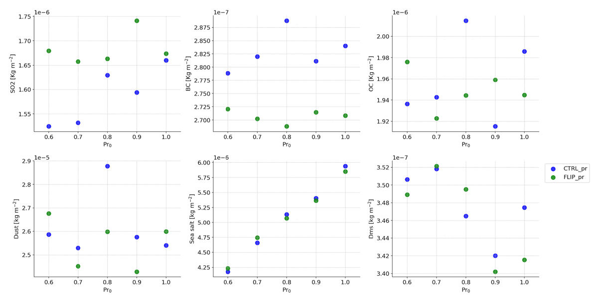
Figure A1
Sensitivity of a one-year simulation of aerosol burdens to variations in the neutral limit Prandtl (Pr0) number, ranging from 1 to 0.6. The default value for Pr0 in both the CTRL and FLIP simulations is 0.8.
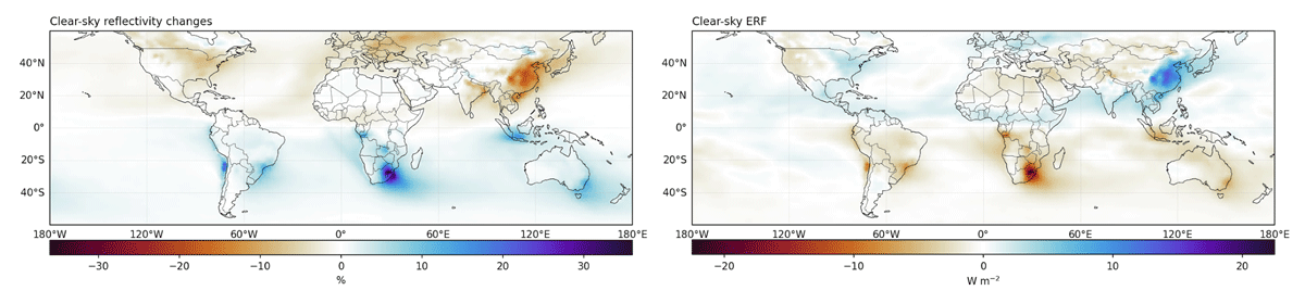
Figure A2
Clear-sky diagnostics between FLIP and CTRL. Left: reflectivity changes (%). Right: clear-sky effective radiative forcing (W m–2).
Table A1
Comparison between the simulations and global observational dataset in terms of cloud properties. Global eight-year annual mean values for key liquid cloud properties using the MODIS COSP simulator in ICON1.3.0-A-HAM2.3 and the MODIS COSP dataset. The OBS used is Nd cloud top (3.7 µm) uses Nd_G18_37 from (Grosvenor and Wood 2018). For the total cloud cover, liquid cloud coverliq, Cloud Effective Radius (CERliq(MC)), Cloud Optical Thickness COTliq, and LWP are from the MODIS COSP (MC) dataset and simulator.
| VARIABLE | OBS | CTRL | FLIP |
|---|---|---|---|
| Nd cloud top (3.7 µm) [cm–3] | 90 | 102 | 98 |
| Total cloud coverMC [%] | 46 | 33.5 | 33.4 |
| Liquid cloud coverMC [%] | 13 | 14.2 | 14.3 |
| CERliq(MC) [µm] | 13.5 | 7.3 | 7.4 |
| COTliq(MC) | 15.3 | 9.2 | 8.8 |
| LWP(MC) [g m–2] | 133.1 | 70.3 | 68.3 |
Competing Interests
The authors have no competing interests to declare.
Author Contributions
Johannes Quaas and Hailing Jia designed the initial experiments. Sabine Hörnig, Jan Kretzschmar, and Alice Henkes implemented the COSP simulator into the ICON-HAM model. Alice Henkes conducted the simulations, performed the analysis, and drafted the initial version of the manuscript. All authors contributed to the interpretation of results, writing, and manuscript revisions.