
1. Introduction
Tracers, such as alkanes (e.g., ethane) or stable isotope ratios, measured alongside the CH4 mole fraction, provide additional information to determine sources of emissions (Basu et al., 2022; Germain-Piaulenne et al., 2024; Rella et al., 2015; Sherwood et al., 2017; Simpson et al., 2012; Turner et al., 2019). Typically, stable carbon isotopic signatures of methane emissions (expressed as δ13CH4) are widely used, from local to global scales to identify biogenic, thermogenic, and pyrogenic emission sources and to better constrain CH4 budget changes (e.g., Al-Shalan et al., 2022; Defratyka et al., 2021; Hoheisel et al., 2019; Lopez et al., 2017; Maazallahi et al., 2020; Menoud et al., 2021, 2020; Phillips et al., 2013; Rella et al., 2015; Röckmann et al., 2016).
However, beyond the biogenic/thermogenic separation, δ13CH4 values of an individual methane emitter from any sector (e.g., landfill, natural gas compressor) can vary widely, depending on numerous factors, such as the CH4 formation process, location, or management practice (e.g., Chanton et al., 2000; Menoud et al., 2022; Sherwood et al., 2017; Whiticar, 1999). Moreover, δ13CH4 signatures for some sectors are spread across a wide range and overlap with δ13CH4 for other sectors (e.g., Bakkaloglu et al., 2022; Fernandez et al., 2022; Menoud et al., 2022; Sherwood et al., 2017). Therefore, a better characterization of δ13CH4 source signatures can improve their source attribution in top-down emission studies (atmospheric observation combined with the inverse modeling), (e.g., Saunois et al., 2020; Varga et al. 2021; Basu et al. 2022). It can also verify bottom-up quantitative approaches, based on process-based models, inventories, and data extrapolation (Lan et al., 2021; Rigby et al., 2012; Schwietzke et al., 2016).
δ13CH4 can be measured for emission plumes downwind of sources from individual sectors (e.g., natural gas, agriculture, landfill) by taking bag/canister samples followed by later measurement in the laboratory (e.g., Bakkaloglu et al. 2021; 2022; Lowry et al. 2020; Townsend-Small et al. 2012; 2016). An alternative is to deploy in-situ instruments, for example, Cavity Ring Down Spectroscopy (CRDS) systems. Such analyser can be equipped with an atmospheric sampling system, called AirCore (air storage tool) (Karion et al., 2010; Rella et al., 2015), to increase number of datapoint, what improves measurements’ precision (Defratyka et al., 2021; Hoheisel et al., 2019; Lopez et al., 2017). Calculating the δ13CH4 source signature (subsequently referred to as δ13CH4 source) is complicated by mixing between source emissions and ‘background’ air, i.e., the atmospheric air remote from any source.
To extract the δ13CH4 source from ambient air samples downwind of a source, Keeling or Miller-Tans methods can be used (Keeling, 1961; Miller and Tans, 2003; Pataki et al., 2003). These methods are based on the principle of mass balance conservation. Both methods use a linear regression to determine δ13CH4 source. As such, the calculation method of choice has an impact on determining a source’s isotopic signature and can potentially bias the determined δ13CH4 source (Miller and Tans 2003; Wehr and Saleska 2017; Zobitz et al. 2006).
Previously, the verification of Keeling and Miller-Tans methods and application of different linear fitting methods was made mostly using synthetic data and theoretical calculation (Wehr and Saleska, 2017; Zobitz et al., 2006) or larger dataset of CO2 respiration (Miller and Tans, 2003; Pataki et al., 2003). Hoheisel et al. (2019) provided a comparison of δ13CH4 source calculated from atmospheric measurements and synthetic data. However, they focused only on the comparison of two linear fitting methods: Ordinary Least Squares method and York fitting. Here, we analyze data from atmospheric, near-source measurements under controlled but realistic field conditions, and include consideration of measurement frequency and instrument uncertainty. Until now, different laboratories use various analytical strategies (e.g. Defratyka et al., 2021; Fernandez et al., 2022; Hoheisel et al., 2019; Lopez et al., 2017; Menoud et al., 2022), that may affect the reported δ13CH4 source and impede inter-laboratory comparison (Menoud et al., 2022; Zobitz et al., 2006).
We analyze isotopic measurement and samples collected within a controlled release experiment to derive a more universal analytical approach for near-source studies of δ13CH4 source. The controlled release experiment aims to be representative of real-life conditions under which existing methane sources, like natural gas infrastructure or sewage emission, are measured. The experiment focused on the validation of several methods for mobile, vehicle-based methane measurements (e.g., Defratyka et al., 2021; Fernandez et al., 2022; Hoheisel et al., 2019; Menoud et al., 2022). Samples collected over five consecutive days of the experiment were analyzed using Isotope Ratio Mass Spectrometry (IRMS) and Cavity Ring Down Spectroscopy (CRDS) measurement techniques (Sect. 2.2), while the CRDS instrument was used both for in-situ sampling using an AirCore tool, and for remote bag analysis after the sample collection. Comparing these three types of measurement techniques, we investigated 1) the influence of the analytical measurement method (IRMS or CRDS), and 2) the impact of increasing measurement frequency for the less precise CRDS. We provide an intercomparison of 1) Keeling and Miller-Tans methods (Sect. 3.1), 2) the impact of chosen backgrounds for Miller-Tans method (Sect. 3.2) and 3) the impact of averaging clusters (Sect. 3.3). Finally, data were re-analyzed using different linear fitting methods (Sect. 3.4).
2. Experimental set-up
2.1. Controlled release set up
The controlled release experiment allows an evaluation of the accuracy and precision of mobile near-source measurements of CH4 emission rates, ethane to methane ratios and δ13CH4. Our experiment took place over 5 days in September 2019 at Bedford Aerodrome, UK. Pure methane was released from a manifolded multi-cylinder pack of twelve cylinders containing 999.6 ± 10.0 mmol mol–1 methane, with an initial pressure of about 200 bars. The impurities in the cylinders came from ethane (48 ± 10 µmol mol–1) and propane (0.149 ± 0.30 µmol mol–1). All 12 cylinders were filled at the same time from the same CH4 source, ensuring δ13CH4 source remained stable over the entire measurement period. The methane release rate varied from 25 L min–1 to 70 L min–1. During the release, CH4 was mixed with ethane (C2H6) in a varying ratio, giving C2H6:CH4 ratios from 0.00 to 0.07. The purity of the C2H6 was 999.9 ± 10.0 mmol mol–1, with impurities mostly from methane (2.27 ± 0.46 µmol mol–1) and propane (7.5 ± 1.5 µmol mol–1). To reach the required CH4 emission rate, CH4 was released simultaneously from all 12 cylinders, using a transportable flow control system (details in Gardiner et al., 2017). Briefly, the flow control system is designed and configured for the creation of ‘real-life’ gaseous emission scenarios, in a range of industrial settings. It allows for validation of methods for emission monitoring applied during typical field conditions. The control system is built on six mass flow controllers (MFC), (Brooks Instrument, Hatfield, PA, USA). Four primary MFCs provide independent emission sources, while two secondary MFCs allow for the introduction of purge and interferant gases into the primary flow. The flow control system is computer operated, allowing for the implementation of pre-written operational programs and the post-test analysis (Gardiner et al., 2017).
Here, the controlled release experiment involved 26 releases, each lasting about 45 minutes. The number of releases per day varied between 2 and 8. The smallest number of releases was conducted during day 1 (3 releases) and day 5 (2 releases). As well as controlling emission fluxes and the ratio of C2H6:CH4, wind speed and direction were measured during all releases. Details of individual gas releases during controlled release experiment are presented in Table A1.
2.2. Measurement technique
During the mobile near-source measurements, the sampling method was based on driving through a plume of CH4. Throughout each release, a vehicle intersected the multiple times plume perpendicular to the wind direction. The controlled release experiment gave the opportunity to validate the mobile laboratories of Royal Holloway, University of London (RHUL) and of the Laboratory for Sciences of Climate and Environment (LSCE). Details of evaluated mobile laboratories are presented in appendix A, with instrument characteristics in Table A2. Briefly, the RHUL mobile laboratory used for this experiment was in operation between 2013 and 2020 (Lowry et al., 2020). This vehicle was equipped with a Picarro CRDS G2301 analyzer, capable to measure mole fractions of CO2, CH4 and H2O, a Los Gatos Research Ultraportable Methane Ethane Analyzer (LGR UMEA), and a manually operated diaphragm pump for filling air sample bags. Three air cylinders were measured and calibrated against the NOAA scale by the Max-Plank Institute for Biogeochemistry Jena, which were used to calibrate the Picarro CRDS G2301 before and after the measurement campaign to the WMO X2004 A CH4 scale (Lowry et al., 2020; France et al., 2016; Zazzeri et al., 2015).
The LSCE mobile laboratory was previously used during mobile studies (e.g., Defratyka et al., 2021), and it is similar to other mobile laboratories equipped with a Picarro CRDS G2201-i (henceforth referred to as CRDS), capable of in-situ measurements of CH4 mole fractions and δ13CH4 (e.g. Rella et al. 2015; Lopez et al. 2017; Hoheisel et al. 2019). The LSCE mobile set-up also comprises of an active AirCore sampler for tripling the sampling frequency during in-situ measurements of δ13CH4 (Defratyka et al., 2021). The LSCE instrument was calibrated using a 3-point mole fraction and isotopic composition calibration, just before shipping the instrument to the UK. After calibration, CH4 mole fractions were reported on the WMO X2004 A scale and δ13CH4 is reported relative to the international Vienna Pee Dee Belemnite (VPDB) standard (Craig, 1957). Due to logistical restrictions, the calibration cylinder or known working gas could not be used during the controlled release experiment. However, an additional working gas was measured in the laboratory before and after the experiment, and no significant drift was observed.
The CRDS measurements were made in a high precision mode, in CO2-CH4 simultaneous mode. CO2 measurement acquisition was kept for additional trouble shooting of analytical artifacts. To resolve short temporal variabilities, the flow rate was adjusted to 100 cc min–1 for faster instrument response during the mobile measurements. Significant cross sensitivities between C2H6 and δ13CH4 in the absorption spectrum have been shown to lead to biases in the measured δ13CH4 by CRDS (details in Appendix A). The effect is inversely proportional to the CH4 mole fraction and proportional to the C2H6 mole fraction in the sample and has been previously quantified (e.g., Rella et al. 2015; Assan et al. 2017).
2.2.1. Collected bag samples measured on IRMS
Air samples analyzed at RHUL were collected by pumping the largest observed enhancement of CH4 plume air into 3 liter Flexfoil® bags (SKC). In total, 21 bags were collected to be measured by IRMS. During the campaign period, at least two bag samples from each CH4 plume, plus a background sample were collected per day. These were measured afterwards in the laboratory, using Picarro CRDS 1301 to determine CH4 mole fraction and using continuous flow gas chromatography isotope ratio mass spectrometry (CF-GC-IRMS Isoprime mass spectrometer with Elementar Trace Gas module, henceforth called IRMS) to determine δ13CH4 (Fisher et al., 2006).
2.2.2. Collected bag samples measured on CRDS
During the three initial releases (two releases over the first day, one release over the second day), bag samples were collected to be measured afterwards on the CRDS instead of using the in-situ AirCore sampler, due to a battery issue with the LSCE mobile laboratory. In total, 10 samples of ambient air were collected in 5 liter Flexfoil® bags (SKC), which allowed for about 20 minutes of measurements using the laboratory-based CRDS. After removing the initial stabilization time, around 15 minutes of measurements were analyzed. The uncertainty was estimated using the standard deviation of measured CH4 and δ13CH4 (1 standard error of 15 minutes of measurements). During this study, bag samples measured by LSCE, were collected only when CH4 was released (C2H6:CH4 = 0.00); thus, the C2H6 on δ13CH4 correction was not applied for bag samples measured by this CRDS.
2.2.3. In-situ CRDS with AirCore
For LSCE in-situ sampling, if the largest CH4 enhancement during the intersection of a CH4 plume reached at least 500 nmol mol–1 above background, the CH4 plume was re-sampled using the air collected and stored in the AirCore (details in Appendix A). AirCore sampling was performed during 12 of the 26 releases. For most of the releases, more than one AirCore sample was collected. In total, 31 AirCore samples were collected.
In the case of AirCore studies, δ13CH4 source were determined both without applying the C2H6 on δ13CH4 correction and with a correction.
2.2.4. Direct δ13CH4 measurement of methane source
To determine δ13CH4 of the source gas, a sample cylinder was filled directly from the multi-cylinder pack after the end of the experiment. Then, the sample was diluted to approximately 600 µmol mol–1 and measured using laser spectrometry. In the next step, 600 µmol mol–1 sample was diluted to 2.5 µmol mol–1 and measured using IRMS at RHUL (Rennick et al., 2021). δ13CH4 measured by laser spectrometry is equal to –41.45 ± 0.06‰ (1 Standard Deviation – 1SD), while δ13CH4 measured by IRMS reached –41.27 ± 0.06‰ (1SD) (Rennick et al., 2021). The true δ13CH4 signature of the cylinder batch, defined as an average δ13CH4 from both instruments, equal to –41.36 ± 0.17‰ was compared with results from samples collected using atmospheric mobile studies.
3. Data processing and source signature determination methods
Figure 1 presents the flow chart of steps to find the best data processing strategy for determination of δ13CH4 source from near-source mobile measurements. Data collected using different measurement techniques (Sect. 2.2) are analyzed, both using Keeling method and Miller-Tans method (Sect. 3.1), while different backgrounds (Sect. 3.2), averaging strategies (Sect. 3.3), and linear fitting methods (Sect. 3.4) are employed.
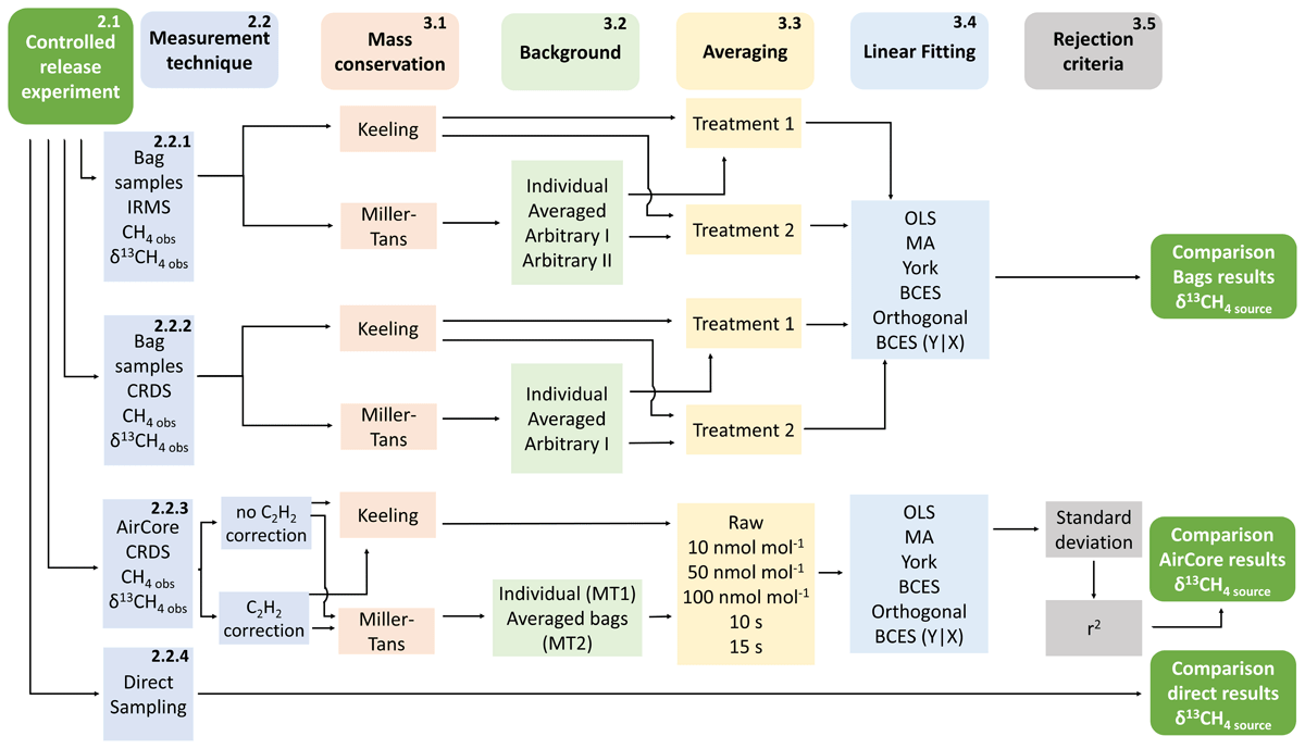
Figure 1
Flow chart of steps to find the best analytical strategy for determination of δ13CH4 source signature, from mobile near-source measurements, based on controlled release experiment. The number in the top right corner corresponds to the methods subsection, where steps are explained in detail.
For bag samples measured on IRMS and CRDS, determination of δ13CH4 source using five regression methods (OLS, MA, York, BCES (Y|X) and BCES Orthogonal) and treatment 1 and treatment 2 averaging approach were implemented, both using Keeling method and Miller-Tans method. For Miller-Tans method, calculations are repeated using different backgrounds: local, averaged, arbitrary I and arbitrary II (Figure 1).
For each AirCore sample, six datasets of distinct clusters (raw data, 10 s, 15 s, 10 nmol mol–1, 50 nmol mol–1 and 100 nmol mol–1) were analyzed using Keeling and Miller-Tans methods. For Miller-Tans method, two different backgrounds were subtracted: individual AirCore background and averaged bag samples background. The analysis was repeated using different regression methods: OLS, MA, York, BCES (Y|X) and BCES Orthogonal (Figure 1). Additionally, the rejection criteria, based on standard deviation and r2 values were applied for each individual AirCore (Sect. 3.5) to select which result should be kept for further analysis and comparison.
3.1. Keeling and Miller-Tans methods
During mobile near-source measurements, the observed CH4 (hereafter CH4 obs) mole fraction and δ13CH4 signature (hereafter δ13CH4 obs) are a mixture of atmospheric background CH4 (hereafter CH4 bckg) and the CH4 source from the source. To determine δ13CH4 source the Keeling or the Miller-Tans methods can be applied (e.g. Hoheisel et al. 2019; Menoud et al., 2020; Defratyka et al., 2021; Fernandez et al., 2022). In the Keeling method (Keeling, 1961; Pataki et al., 2003), δ13CH4 obs is plotted against the inverse of CH4 obs mole fraction and the y-intercept of the fitted linear regression is interpreted as the δ13CH4 source of the observed source:
where subscripts obs, bckg, and source refer to observed, background, and source values. Notably, parameter CH4bckg∙(δ13CH4bckg – δ13CH4source) does not affect δ13CH4 source determined as intercept of Eq. 1, and it can remain as an unknown parameter.
The Miller-Tans method (Miller and Tans, 2003) is another mass conservation approach, where the mole fraction and the isotopic signature of atmospheric background are assumed to be well known. The isotopic signature of the source is represented by the slope of a fitted linear regression, where, after background subtraction, δ13CH4 obs multiplied by CH4 obs mole fraction is plotted against CH4 obs mole fraction:
The Miller-Tans method can be useful to interpret studies, where the Keeling method assumption of stable background is unfulfilled or unknown, e.g., when studies are conducted over a long period of time (Al-Shalan et al., 2022; Lowry et al., 2020).
3.2. Background subtraction for Miller-Tans method
On the small scale, the diurnal variation of CH4 mole fraction can be observed. Additionally, some local CH4 enhancements can exist and affect the background determination. Under these circumstances and regarding available instrumentation, one needs to decide how to define the background, which is defined as a part of the Miller-Tans method. To evaluate the impact of a chosen CH4 bckg mole fraction and δ13CH4 bckg isotopic signature, defined backgrounds are subtracted for the Miller-Tans method. For bag samples measured by IRMS, as a first attempt, an ‘individual background’ was subtracted, defined from a background bag sample collected directly after the release, when bag samples were collected within CH4 enhancement. For example, for all bag samples collected during the first day, the background sample collected on the first day was subtracted. For the next calculation, an ‘averaged background’ is subtracted, which is defined as the average of all background bag samples collected over whole experiment. Next, to verify the sensitivity of Miller-Tans method for a subtracted background, calculations for two arbitrary chosen backgrounds with lower CH4 bckg mole fraction and δ13CH4 bckg than during the experiment were conducted: ‘arbitrary I’ and ‘arbitrary II’ background. For arbitrary I background, CH4 bckg mole fraction is defined as an average global CH4 mole fraction observed in September 2019, equal to 1.871 ± 0.001 µmol mol–1 (Dlugokencky, 2022), while δ13CH4 bckg is defined using value from Brownlow et al., as –47.2 ± 0.2‰ (2017). For arbitrary II background, the CH4 bckg mole fraction is set up the same as the arbitrary I background, but the δ13CH4 bckg set to –42.7 ± 0.2 ‰.
For bag samples measured by CRDS, the Miller-Tans method is implemented three times, while defined backgrounds are subtracted. The backgrounds have been chosen similarly as for the IRMS analysis. Thus, the analysis is implemented three times where individual, averaged, and arbitrary I background are subtracted. The CH4 bckg mole fraction and δ13CH4 bckg for bag samples measured on IRMS and CRDS are presented in Appendix A.
In the case of in-situ AirCore sampling, for the Miller-Tans method, data were analyzed twice to examine possible impact of subtracted background. First, subtracted background is calculated individually for each AirCore, as an average of AirCore background data of an individual AirCore sample, observed directly before and after CH4 obs elevation (defined for later as Miller-Tans 1). Second, averaged background of all bag samples measured on CRDS was subtracted for each individual AirCore sample (Miller-Tans 2) to evaluate sensitivity of Miller-Tans method for subtracted background.
3.3. Data averaging
3.3.1. Data averaging bag samples measured by IRMS and CRDS
In the long-term perspective, bag samples are collected downwind of some sites during multiple visits over a few years (e.g., Lowry et al., 2020). To report δ13CH4 source from multiple visits, determined δ13CH4 source are averaged. Thus, in this study we verify the impact of the chosen averaging strategy on the determined δ13CH4 source. For bag samples under ‘treatment 1,’ δ13CH4 source is calculated separately for each individual day and the final δ13CH4 source is calculated as an average of determined δ13CH4 source for individual days over five consecutive days. This approach is commonly used, however; to quantify its impact, another averaging strategy was tested. In a ‘treatment 2’ averaging approach, the results of bag samples from all releases are treated as one data set and δ13CH4 source and its uncertainty is determined directly from the linear regression. For both treatment 1 and treatment 2 averaging approaches, different data processing strategies were implemented where individual, averaged, and arbitrary background subtraction in the Miller-Tans method were tested.
3.3.2. Data averaging AirCore in-situ sampling
For the AirCore in-situ sampling, the observed δ13CH4 obs fluctuated, which can impact the determined δ13CH4 source. To check if data smoothing (i.e., through averaging) improves the determination of δ13CH4 source, observational data was averaged in clusters before being analyzed. In total, six data sets have been prepared from each AirCore sample and were further analyzed using the Keeling and Miller-Tans methods: raw data, three clusters based on CH4 mole fraction and two time-average clusters (Figure 1). For CH4 mole fraction clustering, clusters with steps of 10 nmol mol–1, 50 nmol mol–1 and 100 nmol mol–1 were used, while for time average clusters, clusters of 10 s and 15 s time averaging were used. Examined clusters were chosen arbitrarily as a compromise between smoothing and potential bias due to over-averaging.
Typically, an individual AirCore sample’s volume allows for collection of 50–80 datapoints. Similar to Hoheisel et al. (2019), AirCore sample measurement errors of individual data points are linearly interpolated based on laboratory tests (details in Appendix A). The interpolated uncertainty of individual points is used as the uncertainty for the clusters of raw data, both CH4 obs mole fraction and δ13CH4 obs signature, for linear fitting methods which require measurement uncertainty as an input (Section 3.4). However, when data points are clustered, based on CH4 mole fraction or time averaging, a total uncertainty of clustered data points is a combination of both the uncertainty of clustering and uncertainty of individual, clustered points (details in Appendix A).
3.4. Linear Fitting method
Both Keeling and Miller-Tans methods rely on linear regression fitting. Potentially, using different linear fitting methods can introduce discrepancies between determined δ13CH4 source and impede its comparison (Menoud et al., 2022; Zobitz et al., 2006). Here we aim the first intercomparison of all broadly used linear regression methods to verify potential biases introduced by different linear fittings: Ordinary Least Squares (OLS) (Defratyka et al., 2021), Major Axis (MA) (Menoud et al., 2022), York fitting (Hoheisel et al., 2019) and Bivariate Correlated Errors and Intrinsic Scatter (BCES) Orthogonal (e.g., Fernandez et al., 2022), adding verification of BCES (Y|X) (Figure 1). Also, we implement comparison between methods including measurements uncertainty (York and BCES) and not including uncertainties (OLS and MA), as OLS method is still the most used linear fitting method.
Most of the tested fittings are calculated using built in packages and functions in the R programming language: OLS using lm() function, MA using lmodel2() function and York fitting using York() function from package IsoplotR. As there is no available package to calculate BCES fitting in R, BCES fitting is calculated using the lnr module in the Python programming language. Throughout the paper, uncertainties of δ13CH4 source determined using different linear regressions are presented as one standard error.
OLS method minimizes the distance only on the y-axis between the fitted line and the data points, using the principle of least squares to minimize the sum of the vertical distances from the regression line, what is also known as model I regression method (Legendre and Legendre, 1998, p. chapter 10). According to Legendre and Legendre (1998), if the error rate on y-axis is more than three times than on x, OLS is the most efficient method to estimate the slope of a linear fitting.
If both x and y variables are not controlled by the researcher or measured with an error, using OLS can cause an underestimation of the slope inferred by the linear regression (Legendre and Legendre, 1998, chapter 10). Thus, the model II linear regression methods are recommended, as they minimize the distance both of x and y from the regression line. The MA method, tested in this study is an example of the model II linear regression. MA method is also known as Orthogonal Distance Regression (ODR) or Deming regression. The MA method minimizes the sum of the squared Euclidean distances (x and y distances) from the regression line. Geometric mean regression (GMR) is another model II linear regression method, but is not tested in this study as it is expected to deliver similar results to the MA method (Zobitz et al., 2006). Details about the standard errors of OLS and MA methods are presented in Appendix A.
In contrast to OLS and MA methods, York fitting (York et al., 2004) and BCES regression (Akritas and Bershady, 1993) allow inclusion of x and y uncertainties. Overall, York fitting can be treated as a general linear regression method, while OLS and MA are special cases valid in particular conditions and can be obtained mathematically from the York fitting method, when appropriate circumstances appear (York, 1966; York et al., 2004). In the York fitting method, the best slope fit is searched iteratively, where the initial slope value is assumed, e.g., using OLS. Then, computations are weighted based on x and y measurement errors. Finally, computations are repeated until differences between iteration are smaller than tolerance level (e.g., 10–15) (York et al., 2004).
The BCES method is a direct extension of the OLS method and was the final linear fitting method evaluated. Within BCES, four sub-methods can be employed: BCES (Y|X), BCES (X|Y), and two symmetric lines: BCES Bisector and BCES Orthogonal (Akritas and Bershady, 1993). BCES (Y|X) assume x as the independent variable. BCES Bisector was shown to be self-inconsistent and should not be used (Hogg et al., 2010). Finally, BCES Orthogonal is a line that minimizes orthogonal distances and should be used when it is not clear which variable should be treated as the independent variable. Our study focuses on the application of BCES Orthogonal, as this method has been broadly implemented in previous studies using IRMS instruments (e.g., Fernandez et al., 2022; Lowry et al., 2020; Zazzeri et al., 2015). Additionally, to examine the difference between the two BCES methods, BCES (Y|X) is also tested, as both methods could be implemented to determine δ13CH4.
To arrive at the final uncertainty of the x- and y-axis, error propagation was applied for both for Keeling and Miller-Tans methods. Details of used error propagation are presented in Appendix A.
3.5. Rejection criteria for AirCore samples
The determined δ13CH4 source is rejected if the standard error of the fitted regression line (intercept for the Keeling method and slope for the Miller-Tans method) is greater than 5‰ (based on the Picarro CRDS performance). Based on previous studies (Defratyka 2021), an additional criterion was applied to the Miller-Tans method, where δ13CH4 source is also rejected if coefficient of determination, r2, is less than 0.85. This additional criterion was not previously applied to the Keeling method, so we examined the variance of the r2 in the Keeling method to determine whether the r2 criterion could also be applied.
Eventually, all retained AirCore δ13CH4 source values from one data processing strategy (mass conservation approach (Sect. 3.1), background (Sect. 3.2), averaging (Sect. 3.3), and linear fitting (Sect. 3.4)) are averaged to obtain a final δ13CH4 source value for each strategy. These final values are then used to compare results from different analytical approaches, presented in the flow chart on Figure 1. Additionally, for releases where bag samples for IRMS and in-situ AirCore sampling occurred simultaneously, the average AirCore results are compared with IRMS results.
4. Results
Since we tested numerous techniques, as presented in flow chart in Figure 1, we present only the most meaningful results in the result section. A more exhaustive analysis can be found in Appendixes B and C. To enable comparison of results we define a reference strategy as the Miller-Tans method with individual background subtraction and the York fitting method, along with treatment 1 averaging for bag samples or raw data for AirCore.
4.1. Measurement technique
For bag samples measured on IRMS, a sample collected during the first day of the experiment, containing 11 µmol mol–1 of CH4, biased results toward more13C enriched values and was rejected from further analysis. Potentially, observed biased came from the necessary sample dilution to obtain CH4 mole fraction in IRMS operational range (details in Appendix B).
Due to the low mole fraction enhancement above the background, bag samples from day 2 exhibited scattered values with bias toward more 13C depleted values, and were rejected from further analysis. Using remaining 18 bag samples measured on IRMS, determined δ13CH4 source varied from –40.55 ± 0.12‰ (day 1) to –39.87 ± 0.10‰ (day 5), reaching treatment 1 average equal to –40.23 ± 0.14‰ and it is treated as a reference value for the other atmospheric results. In the case of samples measured with CRDS, those from day 2 were also rejected from further analysis, thus only bags collected during first day of the experiment (releases 1.1 and 1.2) were analyzed. For in-situ CRDS sampling using the AirCore tool, 3 out of 31 collected samples were rejected, due to CRDS cavity pressure and temperature instability.
Table 1 presents the comparison of determined δ13CH4 source for individual releases, where sampling using two different methods was done simultaneously, and for the averaged δ13CH4 source using treatment 1 averaging for all measurements techniques. Due to better instrument precision and accuracy, δ13CH4 source determined using IRMS has lower uncertainty than CRDS results. From all tested measurement techniques, the uncertainty associated with bags measured by CRDS is the largest.
Table 1
Comparison of direct and averaged results using bag samples measured on IRMS and CRDS (treatment 1 averaging), and CRDS AirCore samples (raw data cluster, without C2H6 correction). The first three rows present comparison for individual releases, where sampling using two different measurement techniques was done simultaneously. Residual between reference IRMS strategy and other analytical strategies for atmospheric measurements. 1 standard error is used as an uncertainty.
| DATE OF SAMPLING | IRMS BAGS YORK FITTING | CRDS BAGS YORK FITTING | RESIDUAL (IRMS—CRDS BAGS) | CRDS AIRCORE YORK FITTING | RESIDUAL (IRMS—CRDS AirCore) |
|---|---|---|---|---|---|
| release 1.1 | –40.60 ± 0.23 | –41.3 ± 8.9 | 0.66 | – | – |
| release 1.2 | –40.56 ± 0.24 | –40.8 ± 3.2 | 0.21 | – | – |
| release 3.3 | –40.45 ± 0.54 | – | – | –40.4 ± 2.8 | –0.09 |
| all 26 releases | –40.23 ± 0.14 | –41.0 ± 6.7 | 0.79 | –41.0 ± 2.7 | 0.81 |
| direct sampling | –41.36 ± 0.17 |
Averaged δ13CH4 source estimates using different data processing strategies, and the result of direct δ13CH4 source measurements, are presented in Figure 2, showing constant δ13CH4 source from IRMS measurements using different data processing strategies. δ13CH4 source measured on CRDS is more variable, depending on chosen data processing strategy (Figure 2). Using York fitting scheme as the reference linear fitting (argumentation in Sect. 4.5), for both CRDS measurement techniques, residuals from IRMS results are smaller than CRDS uncertainties. Thus, results from CRDS and IRMS instruments are in good agreement within the uncertainty. The agreement is observed for δ13CH4 source determined from both individual releases and averaged δ13CH4 source (Table 1).
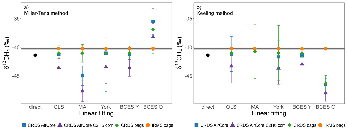
Figure 2
Comparison of direct and averaged results for different linear fitting methods. Bag samples measured on IRMS and CRDS (treatment 1 averaging), and CRDS AirCore samples (raw, non-clustered data) from mobile near-source measurements conducted during controlled release experiment. Results using Miller-Tans with individual background subtracted (left) and Keeling (right) methods are compared. Black line represents IRMS reference value with its uncertainty (gray line). For averaged δ13CH4, uncertainties calculated as 1 standard error. The outlier result for MA linear fitting is not plotted. Compared linear fitting methods: OLS—Ordinary Least Squares, MA- major axis, BCES Y—Bivariate Correlated Errors and Intrinsic Scatter (Y|X) and BCES O—Bivariate Correlated Errors and Intrinsic Scatter Orthogonal.
Direct δ13CH4 source measurements were more depleted (–41.36 ± 0.17‰) comparing to the atmospheric measurements. The uncertainties of direct measurements and IRMS technique are smaller than the observed discrepancy of 1.1‰ between direct and atmospheric IRMS measurements of δ13CH4 source. The averaged CRDS results (both for bags and AirCore samples without C2H6 on δ13CH4 correction) are enriched about 0.3‰ comparing to direct measurements, but due to larger uncertainty of CRDS results, observed discrepancy is irrelevant within uncertainty (Figure 2).
The impact of C2H6 on δ13CH4 correction was tested for all data processing strategies and the same trend is observed for all strategies. Thus, for simplicity the results are discussed and presented on Figure 3 only for non-clustered York fitting strategy. Applying C2H6 on δ13CH4 corrections shifts AirCore values toward more depleted13C values, both comparing to IRMS results and to direct measurement of the cylinder batch. The residual reaches –3.2‰), and –2.05‰), comparing to bags on IRMS and direct measurements, respectively. As observed bias is significant, and deep examination of C2H6 on δ13CH4 correction is out of scope of this study, hereafter we will mostly focus on results from AirCore samples where C2H6 on δ13CH4 correction was not applied.
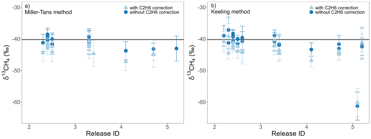
Figure 3
Individual AirCore samples with and without a C2H6 on δ13CH4 correction from mobile near-source measurements conducted during controlled release experiment. Rejection criteria applied. For simplicity, only York fitting, and raw non-clustered data are presented, as the same trend is observed for all data processing strategies. Left: Miller-Tans with individual background subtracted method, Right: Keeling method. δ13CH4 calculated as 1 standard error. Black line represents IRMS reference value with its uncertainty (gray line).
4.2. Keeling and Miller-Tans methods
Estimates of δ13CH4 source determined using Miller-Tans and Keeling methods from bags measured on IRMS demonstrated insignificant difference for all applied linear fittings (Figure 2).
Results from bag samples measured with CRDS, using the York fitting, the δ13CH4 source showed a negligible difference of 0.02‰ between δ13CH4 source values determined using the Miller-Tans and Keeling method. The observed difference in determined δ13CH4 source and its uncertainty varies depending on the chosen linear fitting approach. The largest discrepancy is observed when MA or BCES Orthogonal fittings are used (Figure 2).
For AirCore samples, the determined δ13CH4 source showed a negligible difference of 0.2‰ for York fitting between δ13CH4 source determined using the Miller-Tans and Keeling method. Similar to results from bag samples measured with CRDS, the observed difference of δ13CH4 source and its uncertainty varies depending on the chosen linear fitting approach. The largest discrepancies are observed when MA (–20‰) or BCES Orthogonal (11‰) fittings are used (Figure 2). This trend is consistent regardless of whether a C2H6 correction on δ13CH4 is applied or not (Figure 2).
4.3. Background subtraction for Miller-Tans method
Using four separately defined backgrounds (individual, averaged, arbitrary I, and arbitrary II), no significant differences are observed for δ13CH4 source from bag samples measured with IRMS. For δ13CH4 source determined from bag samples measured with CRDS, where three different backgrounds (individual, averaged, and arbitrary I) were tested, also no impact of subtracted background was observed for all analytical strategies, except for BCES Orthogonal. A similar dependency was observed for δ13CH4 source determined from AirCore samples, where individual and averaged backgrounds were subtracted. Tables of determined δ13CH4 source are presented in Appendix B for bag samples and in Appendix C for AirCore samples.
4.4. Data averaging and clustering
4.4.1. Data averaging bag samples measured by IRMS and CRDS
For analysis of bag samples measured on IRMS, the δ13CH4 source reached –40.23 ± 0.14‰ using treatment 1 averaging, and –40.18 ± 0.05‰ using treatment 2 averaging. Thus, the observed discrepancy is insignificant for the IRMS study. For samples measured with CRDS, the residual difference between treatment 1 and 2 averaging was 0.3‰), and it is also insignificant.
4.4.2. Data averaging AirCore in-situ sampling
Subsequently, the impact of clustering data (using both CH4 mole fraction and time averaging clusters) on the final, averaged δ13CH4 source for AirCore samples, is presented on Figure 4. The details about clustering impact for analysis using different mass conservation methods and linear fittings can be found in Appendix C. Overall, clustering causes a changeable bias for AirCore samples, which depends on the chosen clustering strategy and the linear fitting. Additionally, clustering increases the uncertainty of the final averaged δ13CH4 source. Furthermore, depending on the clustering method and the linear fitting, the amount of rejected individual AirCore samples varies. For example, for York fitting, for 50 nmol mol–1 and 100 nmol mol–1 CH4 mole fractions clusters, only one individual AirCore result remains for each cluster. The largest discrepancies between raw and clustered data are observed for the MA and BCES Orthogonal linear fitting methods, possibly due to forced symmetry applied in both methods, with δ13CH4 source reaching up to –7.6 ± 2.4‰ (Figure 4).
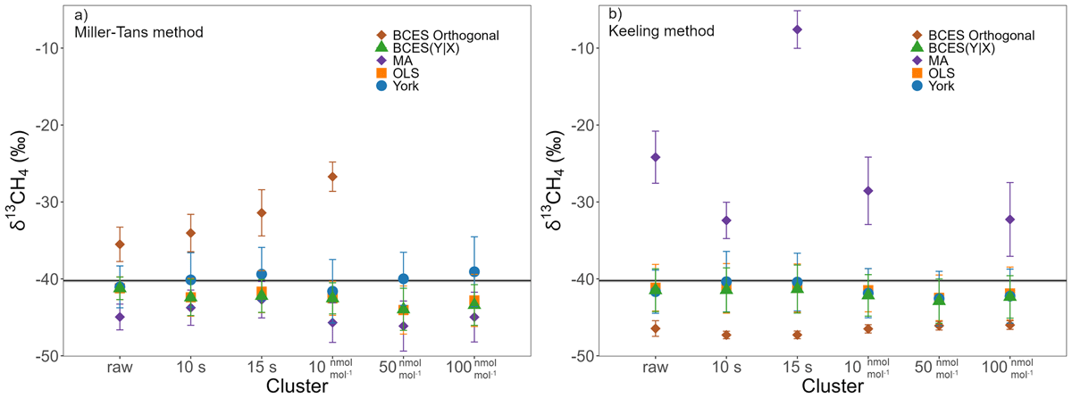
Figure 4
Comparison of averaged CRDS AirCore samples for different cluster averaging from mobile near-source measurements conducted during controlled release experiment. C2H6 correction was not applied. Results using Miller-Tans with individual background subtracted (left) and Keeling (right) methods are compared. δ13CH4, uncertainties calculated as 1 standard error. Black line represents IRMS reference value with its uncertainty (gray line). Compared linear fitting methods: OLS—Ordinary Least Squares, MA- major axis, BCES Y—Bivariate Correlated Errors and Intrinsic Scatter (Y|X) and BCES O—Bivariate Correlated Errors and Intrinsic Scatter Orthogonal.
4.5. Linear fitting
Regarding the results from bag samples measured on IRMS, differences between determined δ13CH4 source using different fitting methods are insignificant (Figure 2). The largest uncertainty is observed for MA linear fitting, where uncertainty is calculated from 95% confidence intervals converted to standard error. The smallest uncertainty is observed for York fitting for both averaging approaches.
In the case of bag samples measured with CRDS, differences between determined δ13CH4 source using different fitting methods are insignificant, except for results where BCES Orthogonal was used (δ13CH4 source equals to –36.9 ± 3.0‰) (Figure 2). For bag samples measured on CRDS, the largest uncertainties are observed for MA and York linear fitting.
For AirCore samples, for OLS, York, and BCES (Y|X) methods, insignificant differences were observed between the Keeling and the Miller-Tans method with two distinct backgrounds, considering raw data clustering (Table 2). The results from these three linear fittings are in good agreement within each other, indicating them as good methods for AirCore data treatment. Similar to bag samples measured with CRDS, larger, and significant discrepancies were observed using MA and BCES Orthogonal methods, reaching –45.0 ± 1.7‰ and –35.5 ± 2.3‰), for raw data. Notably, only for the BCES Orthogonal fitting, the results from Miller-Tans methods with two differently defined backgrounds were significantly different.
Table 2
CRDS AirCore samples for raw cluster data. nAirCore represents number of AirCore samples used to determine averaged δ13CH4 after applying rejection criteria. C2H6 on δ13CH4 correction not applied; one standard error is used as an uncertainty.
| LINEAR FITTING | δ13CH4 ± U(δ13CH4) (‰) | nAirCore KEELING METHOD | nAirCore MILLER-TANS 1 | nAirCore MILLER-TANS 2 | ||
|---|---|---|---|---|---|---|
| KEELING METHOD | MILLER-TANS METHOD 1 | MILLER-TANS METHOD 2 | ||||
| OLS | –41.1 ± 3.0 | –41.2 ± 1.5 | –41.2 ± 1.5 | 22 | 12 | 12 |
| MA | –24.2 ± 3.4 | –45.0 ± 1.7 | –45.0 ± 1.7 | 2 | 12 | 12 |
| York | –41.7 ± 2.8 | –41.0 ± 2.7 | –40.9 ± 2.1 | 21 | 12 | 12 |
| BCES Orthogonal | –46.5 ± 1.0 | –35.5 ± 2.2 | –39.8 ± 1.9 | 19 | 9 | 12 |
| BCES (Y|X) | –41.4 ± 2.8 | –41.2 ± 1.5 | –41.2 ± 1.5 | 25 | 12 | 12 |
4.6. Rejection criteria
Previous research using the Miller-Tans method proposed to reject individual AirCore sample results if their uncertainty is greater than 5‰), and if r2 is less than 0.85 (Defratyka et al., 2021). The fraction of rejected AirCore predictably varied with the data processing strategy (Table 2 and more details in Appendix C). For example, using the reference analytical strategy, 12 out of the 28 AirCore samples remained, after applying the rejection criteria.
We investigated whether the same rejection criteria can be applied to the Keeling method. For the CRDS AirCore studies, the r2 values remain scattered, regardless of whether determined δ13CH4 source agreed with IRMS reference value or not. Also, r2 remains systematically low, mostly ranging between 0.1 and 0.3. Thus, it was not possible to find a satisfying r2 rejection criterion for Keeling method. Applying only the uncertainty criterion leads to fewer rejections and a wider spread of δ13CH4 source among individual AirCore samples using the Keeling method, which therefore increases the uncertainty of the final, averaged δ13CH4 source (Figure 4).
5. Discussion
5.1. Comparison with previous studies
A few studies have been conducted to find the best strategy for applying the Keeling or the Miller-Tans methods to determine isotopic signatures, and they focused mostly on synthetic data or continuous measurements of CO2 (Miller and Tans, 2003; Pataki et al., 2003; Wehr and Saleska, 2017; Zobitz et al., 2006). Furthermore, Hoheisel et al. (2019), focused on atmospheric CH4 measurements, using both CRDS AirCore sampling and synthetic data to compare use of OLS and York fitting during the application of the Keeling and Miller-Tans method. Pataki et al. (2003) concentrated on the application of the Keeling method for δ13C of CO2. However, as they highlighted in their paper, this method can be used also for other gas species or isotopes, where each application has its own constraints. Pataki et al. (2003) and Miller and Tans (2003) recommend using the model II (e.g. MA) fitting method for mass conservation because the OLS method could introduce a systematic bias, especially if the linear fitting r2 value is low. However, Zobitz et al. (2006) showed that model II can also introduce some bias if the range of the CO2 mole fraction is low (e.g., CO2 enhancement above background is lower than 20 µmol mol–1) and if variability on the x-axis is much lower than in the y-axis. Geometric mean regression (GMR) is another model II linear regression method that was not tested in our study, as it is expected to yield similar results to the MA method (Zobitz et al., 2006). In our study, we observed bias in the MA method for CRDS studies, where the uncertainty and fluctuation of the measured δ13CH4 obs were greater than those for CH4 obs mole fractions. As advised by Hoheisel et al. (2019), we focused on releases where the measured CH4 mole fraction exceeded the background mole fraction by at least 0.5 µmol mol–1. This provided a signal-to-noise ratio large enough to avoid introducing biases in high precision IRMS measurements using the model II method. However, bias due to low signal-to-noise ratio can occur when observing lower enhancements. This is typically the case for measurement stations conducting continuous measurements located at some distance from the source.
Hoheisel et al. (2019) focused on the comparison of the Keeling and Miller-Tans methods, using OLS and York fittings, for CH4 obs AirCore and synthetic data. Regarding the comparison of measurement techniques, they obtained identical results for the Keeling and Miller-Tans methods when using York fitting. Using OLS fitting, they observed differences from –2‰ to 2‰ for individual AirCore samples between the Keeling and Miller-Tans methods. Hoheisel et al. (2019) showed that for AirCore studies, the results from York fitting fall between results obtained using OLS with the Keeling or Miller-Tans method for 90% of the measurements. In their study, results from York and OLS are nearly the same, but both show larger differences from the true, modeled value than from each other. The observed discrepancy between the fitted and true value reached <0.2‰ These results are consistent with our study, where we did not observe significant differences between York and OLS fittings and similar discrepancies between AirCore samples and direct δ13CH4 source. Moreover, Hoheisel et al. (2019) investigated the influence of averaging time, examining intervals up to 1 minute. Using synthetic data, they demonstrated no significant differences between raw and 15 s averaged. They also observed improved precision of the measurements when averaging over 1 minute, but this did not enhance the determination of δ13CH4 source. This contrasts with our results from mobile measurements, where we observed a varying bias introduced by data averaging, using different clusters, which worsens the determination of the final δ13CH4 source (Figure 4).
We found that implementing a C2H6 correction on δ13CH4 (as described in other studies) introduces a possible bias, resulting in the final averaged δ13CH4 to be more13C depleted than calculated from IRMS measurements or from measurements made directly from the cylinder batch. To our knowledge, this is the first study to directly compare CRDS AirCore results with δ13CH4 source determined from bag samples measured on an IRMS and direct source sampling, providing evidence to exclude a C2H6 correction for measuring δ13CH4 in these types of samples. Previous studies that implemented a C2H6 correction focused solely on CRDS AirCore measurements, without the comparing them to independent C2H6-interference free measurements (Assan et al., 2017; Hoheisel et al., 2019; Lopez et al., 2017; Rella et al., 2015).
Finally, several studies, including Wehr and Saleska (2017) and Hoheisel et al. (2019), proposed using York fitting to determine δ13CH4 source, as it is the most general regression method, which also accounts for uncertainties of both the x- and the y-axis. Based on Monte Carlo simulations, used to determine the isotopic signatures of CO2, Wehr and Saleska (2017) presented that York fitting produces the closest realistic results, compared to OLS and GMR methods. Their conclusion aligns with our study, as the York fitting method consistently provides robust results for all examined analytical approaches. Additionally, we observe smaller discrepancies between the OLS and York fitting methods compared to the studies of Wehr and Saleska (2017). This can be explained by the larger CH4 enhancements relative to CO2 enhancements experienced in our study compared to theirs. Notably, we also tested the BCES linear fitting using two sub-methods: BCES (Y|X) and BCES Orthogonal, which had not been previously tested for atmospheric applications. We demonstrated that the choice of linear fitting method does not affect IRMS results. For AirCore samples, BCES (Y|X) results are in good agreement with York fitting results, whereas BCES Orthogonal introduces significant bias and should not be used for AirCore samples.
5.2. Possible improvements and further applications
Based on our study, several analytical details warrant special attention during the determination of δ13CH4 source. We observed that individual AirCore values for samples collected on days 4 and 5 of the controlled release experiment were more depleted compared to samples collected from days 2 and 3 (Figure 3) and from the reference IRMS value. It is possible that an unnoticed issue, such as a leak, may have occurred during those days. Therefore, we recommend measuring calibration and working target gases on each measurement day, both before and after the fieldwork.
We observed about a 1.1‰ discrepancy in IRMS results between atmospheric and directly determined δ13CH4 source. This discrepancy could be caused by different conditions in which direct and atmospheric samples were collected. For atmospheric studies, the gas was released over 45 minutes from the cylinder at high rates (up to 70 l min–1) and was sampled in a downwind plume up to 250 m from the release position. For direct sampling, gas was transferred from cylinder batch to 10 L cylinder in less than two minutes. During the controlled release experiment, we did not observe significant differences or trends between atmospheric δ13CH4 source determined during different releases, even when CH4 flow rate, wind speed, or wind direction varied. These physical phenomena alone only impact the dispersion characteristic of CH4 from the source to the sampling location, without any plausible mechanism for isotopic fractionation within the boundary layer on these short timescales. Further studies on possible isotopic fractionation during gas release are planned in the future to verify observed discrepancy.
In our study, we focus entirely on finding the best data processing strategy for near-source mobile measurements to determine δ13CH4 source. However, we anticipate that the results can be generalized to other applications where similar isotopic mixing lines are appropriate. For example, the same conclusions should apply for the determination of δD-CH4 and stable isotope ratios of CO2. Also, our conclusions should be applicable for continuous isotopic measurements, both for CO2 and CH4. Before expanding our conclusion to other isotopes or continuous measurement studies, it is important to consider that the range of observed mole fractions, signal-to-noise ratios, precision, and variability of the y-axis could potentially introduce biases depending on their magnitudes and on the chosen fitting methods. Based on our study, York, and BCES (Y|X) are good candidate methods to apply in different contexts, as they exhibited the least variability and incorporate uncertainties of the x- and y-axis. Furthermore, establishing rejection criteria for individual applications, such as the size of uncertainty or the r2 parameter, can identify outliers and improve the accuracy and precision of determining δ13CH4 source isotopic signatures.
6. Conclusions and recommendations
Our study aims to find the most robust data processing strategy for determining δ13CH4 source isotopic signatures from mobile measurements, while eliminating the need to choose between biased methods or switch between methods depending on the conditions. With the increasing popularity of CRDS instruments for measuring source signatures, it is crucial to evaluate comparatively the performance of both IRMS and CRDS for determining δ13CH4 source. The novelty of the study is the comprehensive inter-comparison between atmospheric studies of δ13CH4 using (i) bag sampling measured afterwards both by IRMS and CRDS, (ii) in-situ CRDS with an AirCore storage tool under controlled release conditions. Also, we focused on intercomparison of different analytical strategies used in atmospheric studies of δ13CH4 source. We tested aspects not detailed in previous studies, such as background subtraction, data averaging, and BCES linear fitting. To achieve this, we focused on data from a controlled release experiment, which simulates real-life methane point sources, such as leaks in natural gas infrastructure. This approach enables the validation and implementation of conclusions from studies primarily focused on synthetic or CO2 data (Miller and Tans, 2003; Pataki et al., 2003; Wehr and Saleska, 2017; Zobitz et al., 2006).
The chosen mass balance approach and linear fitting method do not significantly affect IRMS results (Figure 2). The high precision and accuracy of IRMS instruments lead to a more reproducible estimation of the δ13CH4 signature than from CRDS measurements. There is no significant difference observed with background subtraction for the Miller-Tans method; however, for the consistency, individual backgrounds should be subtracted. Bag samples collected on different days should not be treated as one dataset. Instead, δ13CH4 source should be calculated for individual days and then averaged.
In contrast, δ13CH4 source measurements are more sensitive to data processing choices for CRDS than for IRMS measurement technique. Estimates of δ13CH4 source determined using in-situ CRDS AirCore measurements agrees well with the IRMS results, when York fitting method is used. The addition of an AirCore unambiguously provides more robust results and should be implemented for in-situ CRDS measurements.
For CRDS AirCore studies, we recommend using the Miller-Tans method, with the subtraction of the individual backgrounds. To achieve robust and accurate results, raw, non-clustered data should be analyzed. For consistency, we recommend using either York or BCES (Y|X) fitting methods for both IRMS bag samples and CRDS AirCore, as they include the uncertainty of measurement points and give the most consistent results. The OLS method can also be applied to determine δ13CH4 source, as differences between York, BCES (Y|X), and OLS fitting methods are not significant within the uncertainty range. However, in the cases of lower CH4 range or higher uncertainty in the measured δ13CH4 source, the discrepancy between York and OLS methods may increase. For CRDS AirCore studies, we strongly discourage the use of the MA and BCES Orthogonal methods, as their forced symmetry introduces varying biases (Figure 4). Adhering to these recommendations will reduce the risk of obtaining inaccurate and imprecise δ13CH4 source isotopic signatures.
The conclusions of our work provide a robust starting point for other applications that utilize isotopic mixing lines. However, the range of observed mole fractions, signal-to-noise ratios, and precision and fluctuation of isotopic signatures have the potential to introduce biases depending on their magnitude and the chosen data processing strategy. Thus, as demonstrated in this study, the applied data processing strategy must be chosen carefully.
Data Accessibility Statement
The data that support the findings of this study are openly available in Defratyka, Sara (2023), ‘Dataset: Statistical evaluation of methane isotopic signatures determined during near-source measurements,’ Mendeley Data, V1, doi: 10.17632/vfbbdvp9w2.1 at https://data.mendeley.com/datasets/vfbbdvp9w2/1.
Additional File
The additional file for this article can be found as follows:
Supplement Information
Appendix A to C and Supplementary References. DOI: https://doi.org/10.16993/tellusb.1878.s1
Funding Information
This research has been supported by the European Union’s Horizon 2020 research and innovation program (Marie Skłodowska-Curie grant no. 722479).
The controlled release experiment was part of the NERC grant New methodologies for removal of methane from the atmosphere (NE/P019641/1), which also funded the LGR UMEA instrument used in these experiments. RHUL participation in the experiment was funded by the NERC Equipt4Risk project (NE/R017360/1).
TA and CR acknowledge funding from 21GRD04 isoMET. 21GRD04 isoMET has received funding from the European Partnership on Metrology, co-financed from the European Union’s Horizon Europe Research and Innovation Programme and by the Participating States.
Competing Interests
The authors have no competing interests to declare.
Author contributions
S.M.D: Writing—original draft, Conceptualization, Visualization, Methodology, Validation, Formal analysis, Data curation, Investigation. J.L.F: Conceptualization, Methodology, Investigation, Data Curation, Writing—review and editing. R.E.F: Conceptualization, Methodology, Validation, Resources, Writing—review and editing. D.L.: Conceptualization, Methodology, Validation, Resources, Writing—review and editing. J.M.F: Investigation, Data Curation, Formal analysis, Writing—review and editing. S.B: Investigation, Data Curation, Writing—review and editing. C.Y.K: Supervision, Methodology, Validation, Resources, Writing—review and editing. J.D.P: Supervision, Validation. P.B: Supervision, Conceptualization, Methodology, Validation, Resources, Writing—review and editing. T.A: Supervision, Methodology, Validation, Writing—review and editing. C.R: Methodology, Validation, J.H: Conceptualization, Methodology, Validation, Investigation, Writing—review and editing. N.Y: Conceptualization, Methodology, Validation, Investigation. E.G.N: Writing—review and editing.