
1. Introduction
The lowest part of the atmosphere, the so-called Planetary Boundary Layer (PBL), is where the Earth’s surface exchanges energy, mass and momentum with the atmosphere (Stull, 1988). The structure and diurnal evolution of the PBL height (PBLH) regulates the dispersion of air pollutants and aerosol particles contained within the layer (Seinfeld, 2003; Singh and Kumar, 2022; Haywood, 2021) having strong impacts on climate, ecosystems and health (Seinfeld and Pandis, 2016, IPCC 2021). The PBLH is influenced by the thermal expansion of air masses adjacent to the surface and thus, tends to follow the diurnal cycle of sunlight: increasing during morning hours, becoming maximum around local noon hours, gradually decaying in the afternoon, and becoming minimum after sunset and during the night. These diurnal PBLH changes affect the PBL volume, hence primary air pollutants emitted within it tend to be diluted during daytime and concentrated at nighttime (Duc et al., 2022), although this may vary considerably in urban regions and near intense aerosol sources (e.g., Foskinis et al., in review). Monitoring the temporal variation of the PBLH with high spatial and temporal resolution provides constraints that can significantly improve air quality assessment and forecasting (Illingworth et al., 2019).
Measuring the PBLH is challenging because it is not strictly defined and can also be estimated with many methods; because of this, the PBLH is inherently subject to uncertainty (Kotthaus et al., 2023). In-situ determination of the PBLH can be done with radiosondes and airborne platforms (e.g., airplanes, helicopters, UAVs, tethered balloons). Remote sensing of PBLH is based on aerosol/wind lidars (Kokkalis et al., 2020), microwave radars, ceilometers (Tsaknakis et al., 2011), sodars, and microwave radiometers (Emeis, 2011).
In this study, we adopt the usage of the Doppler lidar technique, which enables detection of vertical profiles of aerosols as well as their velocity as “tracers” of the air mass movements. This technique, based on the detection of the minimum of the gradient of the backscattered elastic lidar signal vertical profile or on the vertical wind velocity w profile, can provide the PBLH with very high spatial (a few meters) and temporal (a few seconds) resolution (Wang et al., 2021; Duc et al., 2022).
It is well established (e.g., Milne and Taylor, 1922; Taylor, 1935) that the vertical size of a growing turbulent plume is proportional to the standard deviation of the updrafts (σw), hence mixing intensity. Given that the PBL is characterized by intense mixing, vertical measurements of σw can be used to determine the extent of the lower atmosphere and PBL, and changes thereof from transitioning inside and out of the PBL. Based on this approach, Kaimal et al. (1976), Tucker et al. (2009), Pearson et al. (2010), Barlow et al. (2011), Träumner et al. (2011), and Schween et al. (2014) determined the PBLH, where the σw values fall below a characteristic threshold ranging between 0.17 m s–1 and 0.40 m s–1. This large variation of the σw threshold may reflect uncertainties in the retrieval of the vertical velocity, or simply the natural variability of the PBL characteristics in different environments. According to Schween et al. (2014), a ±25% change in the threshold translated to a ∓7% change in the PBLH.
In the case of the orographic environments, the PBLH estimation poses a particular challenge, given its complex structure owing to the topography and the large diurnal forcing. The wind Doppler lidar technique can constrain the PBLH with unprecedented temporal and spatial resolution (Emeis, 2011). In this study, we deploy the HALO lidar system to derive a proper σw threshold value for the PBLH determination at the (HAC)2 station at Mount Helmos (Greece), using additionally in situ observations of the annual variations of the PBL dynamics, and ultimately determine the time periods that the (HAC)2 station (and corresponding orographic clouds) is influenced exclusively by PBL or FTL air masses, even a combination of those.
2. Methodology and Experimental site
The (HAC)2 station is located at the top of the Helmos mountain in the Peloponnese, at an altitude of 2,314 m a.s.l. (37.984033 °N, 22.196060 °E; c.f. Figure 1). It stands as the sole high-altitude facility for atmospheric research in the Eastern Mediterranean region, dedicated to probing the aerosol physico-chemical characteristics and climate-related gases (e.g., CO2, CH4, H2O, etc.). It has been established and operated by the ENvironmental Radioactivity & Aerosol technology for atmospheric and Climate impacT Lab (ENRACT) of the National Centre for Scientific Research Demokritos (NCSRD) since 2015. According to Collaud et al. (2018), (HAC)2 has very low PBL-TopoIndex values, which means that the influence of the PBL is statistically low compared to other high-elevation sites.
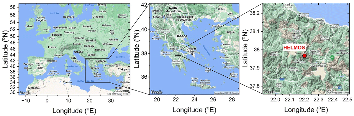
Figure 1
The study area (left), the sub-domain over Greece (middle), and the regional area around (HAC)2 is marked by a red dot.
The dataset used in this study has been obtained during the international Cloud-AerosoL InteractionS in the Helmos background TropOsphere (CALISTHO) Campaign (https://calishto.panacea-ri.gr/), which took place at the Helmos mountain, from September 2021 to March 2022, to study the cloud microphysical properties using a synergy of in situ and remote sensing techniques.
The origin of the sampled air masses at (HAC)2 is initially characterized through in situ measurements by a set of instruments consisting of: an aethalometer (AE31) for measuring the equivalent black carbon (eBC) concentration, a nephelometer (TSI 3563) to measure the light-scattering coefficient of aerosol particles at multiple wavelengths, a Wideband Integrated Bioaerosol Sensor (WIBS-5/NEO) to measure the presence of biological particles (pollen, bacteria and fungi), and a Scanning Mobility Particle Sizer (SMPS) to determine the total concentration of particles (NTotal), as well as the concentration of particles between 90 and 800 nm (N90–800 nm). Meteorological data (ambient temperature and pressure, Relative Humidity (RH), and horizontal wind) at surface, are provided by a meteorological station located at (HAC)2, while the absolute humidity (q) was calculated based on the ambient temperature and pressure (Wallace and Hobbs, 2006).
The strong contrast between the PBL and FTL air masses, using all these in situ parameters as proxies, is used to constrain when the PBLH crosses the (HAC)2 altitude. A wind Doppler lidar, placed at the “Vathia Laka” (VL) location (37.999473 °N, 22.193391 °E) –1.7 km away and 500 m below (HAC)2, provided the vertical profiles of σw throughout the atmospheric column. Using this setup, we were able to follow the vertical movements of air masses between (HAC)2 and VL and measure the σw at the level of (HAC)2 thus, identifying when this site is above or inside the PBL. The latter is then used to determine the appropriate σw threshold for defining the PBLH.
2.1 Instrumentation
We present below the in situ and remote sensing instrumentation deployed to study the PBLH variation during the CALISHTO Campaign.
2.1.1. Aethalometer (AE31)
The TSI 3563 nephelometer measures the scattering coefficient of the dried aerosol particles (RH below 40%), after a PM10 inlet, at three different wavelengths (450, 550 and 700 nm). The aethalometer AE31 measures the equivalent black carbon (eBC) concentration based on Hansen et al. (1982) and Petzold et al. (2013). Given that the black carbon primarily stems from anthropogenic fossil fuel emissions (the wildfire cases are excluded from our study) within the PBL, we can use the eBC as an index to ascertain the conditions under which the (HAC)2 resides either within the PBL or the FTL. This determination depends on whether the eBC concentration obtains large or small values, respectively (Lund et al., 2018; Motos et al., 2020). The instrument operates after a PM10 inlet at dry conditions (RH below 40%).
2.1.2 Nephelometer (TSI 3563)
The TSI 3563 nephelometer, measures the scattering coefficient of the dried aerosol particles, at three different wavelengths. The nephelometer provides the aerosol backscatter coefficient and by using the Beer-Lambert law it calculates the aerosol total extinction coefficient at 450, 550 and 700 nm. Here, the aerosol scattering intensity is again used as a proxy to evaluate whether the (HAC)2 is within the PBL or FTL. Given that increased aerosol concentrations are typically found within the PBL, the relevant total scattering coefficient tends to obtain large values (Farah et al., 2018) when (HAC)2 is within the PBL. Moreover, in this study, we used the aerosol total scattering and backscattering coefficients at 550 nm (sc550 and bc500, respectively).
2.1.3. WIBS-5/NEO (WIBS)
The wideband integrated bioaerosol sensor-New Electronics Option (WIBS-5/NEO, Droplet Measurement Technologies) characterizes and records the concentration of total and fluorescent aerosol particles with size between 0.5 to 30 μm (optical) diameter. The fluorescent particles are classified in three channels depending on their fluorescent properties: the FL1 channel, with excitation wavelength at 280 nm and fluorescence detection at 310–400 nm, the FL2 and FL3 channels with laser excitation at 280 and 370 nm and detection spectral region at 420–650 nm, respectively (Perring et al., 2015; Savage et al., 2017), then are tuned to detect the fluorescence from three classes (A, B and C) for ubiquitous biological fluorophores, including tryptophan-containing proteins, NAD(P)H co-enzymes and riboflavin (Kaye et al., 2005; Savage et al., 2017; Pöhlker et al., 2012). When the aerosol particles fluoresce in more than one class, the extra classes are defined as AB, BC, AC, and ABC, respectively. Given that the pollen, used as a tracer to define the PBL extend over the (HAC)2, gives strong fluorescence at BC and ABC (Hernandez et al., 2016), we studied only those two classes.
The mean background signal plus 9-times its standard deviation (measured from routinely performed forced-trigger tests) is used as the detection limit for particle fluorescence. Given that non-biological particles, such as some black carbon and dust particles, may fluoresce in one of these channels (Toprak and Schnaiter, 2013), the aerosol particles showing fluorescence in all three channels are most likely to be of biological origin (e.g., pollen, bacteria, and fungi) (Savage et al., 2017).
2.1.4 Scanning Mobility Particle Sizer (SMPS)
The Scanning Mobility Particle Sizer (SMPS) measures the aerosol number size distribution, every 5 minutes. The SMPS employs a Vienna-type DMA (electrode length 28 cm) with a condensation particle counter (CPC model 3772, TSI Inc.) to measure particles ranging from 10 to 800 nm. The SMPS operates at a sheath flow rate of 5 L min–1 and an aerosol flow rate of 1 L min–1. Before detection, the ambient aerosol enters the DMA and passes through an 85Kr neutralizer to achieve an equilibrium charge distribution. Lastly, both the aerosol sample flow and the sheath air flow get dried below 40% relative humidity using Nafion dryers, while the temperature, relative humidity, and pressure inside the instrument are continuously monitored during the sampling process.
2.1.5 Wind lidar system and PBLH retrieval
During CALISHTO, a HALO Photonics StreamLine XR Doppler lidar was deployed by the Finnish Meteorological Institute (FMI) at the VL site. The HALO is a pulsed Doppler lidar and operates at 1.5 μm wavelength (Pearson et al., 2009). HALO reports both attenuated backscatter and radial velocity at 30 m range resolution; in vertical stare mode, excluding clouds and precipitation, the measured velocity corresponds to the vertical velocity of the surrounding air masses, i.e. vertical wind velocity (w) (Henderson et al., 2005). Vertical stare was configured at 5 s integration time, alternating between co- and cross-polar receiver. In addition to the vertical stare, velocity azimuth display (VAD) scans were performed to retrieve horizontal winds (Browning and Wexler, 1968). Range of the HALO lidar is 12 km, but in practice in staring mode the maximum range of useful signal varies from 2 to 3 km depending on the atmospheric aerosol load.
Additionally, to minimize instrumental noise effects on the retrieved σw, we digitally filtered the HALO lidar data using the technique proposed by Barlow et al. (2011), Newsom and Krishnamurthy (2020), by excluding the data characterized by a signal-to-noise ratio (SNR) lower than –20 dB. Secondly, we calculated the standard deviation σw within a 30-minute time-moving window (Lenschow et al., 2012, Schween et al., 2014) for each height level.
The average time window of 30 min describes the time needed by a convective air plume to travel up and down within a well-mixed PBL. Considering that a plume has on average, an ascent speed of 1 m s–1 and that a typical mixing layer at (HAC)2 is about 1 km, the average time interval is about twice the mixing timescale. This time window is also typical for the derivation of turbulent fluxes from eddy covariance stations according to Schween et al. (2014).
Finally, we calculated the σw at the (HAC)2 altitude, and we combined the in situ measurements from the SMPS, AE31, TSI 3563, WIBS, and meteorological parameters to derive a threshold value of σw to delineate whether (HAC)2 is confined within the PBL or above (in the FTL), or in a transition zone between these two regions.
3. Experimental Results
3.1 Results Overview
Figure 2 presents the RH, T, and horizontal wind velocity recorded at (HAC)2. As previously mentioned, the aerosol scattering (sc550) and backscattering (bc550) coefficients were derived from the Nephelometer; the N90–800 nm and the NTotal were derived from the SMPS data; the eBC concentrations were derived from the Aethalometer data; the AB and ABC signals were obtained from WIBS; while the σw was derived from HALO at the level of (HAC)2.
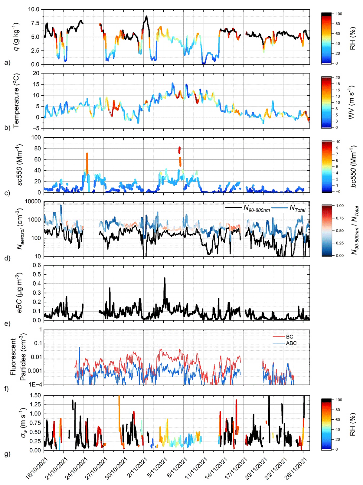
Figure 2
Timeseries of a) q (g kg–1) and RH (%), b) ambient temperature (oC) and horizontal wind velocity (m s–1), c) scattering coefficients sc550 and bc550 (Mm–1), d) N90-800 nm, Ntot (cm–3) and N90–800 nm/Ntot, e) eBC (μg m–3), f) fluorescent particles BC and ABC (cm–3), and f) σw (m s–1), as measured by the synergy of in situ and remote sensing techniques at the (HAC)2 height level between 18 October to 26 November 2021.
Under cloud-free conditions at (HAC)2, the sampled air masses contain low levels of moisture (q: 0–2.5 g kg–1, RH: 0–40%) and σw usually varies between 0–0.25 m s–1. In these cases, the fine particles (below 90 nm) dominate the aerosol number (N90–800 nm/NTotal < 0.25), and N90–800 nm varies between 0 and 120 cm–3 and the aerosol scattering coefficients (sc550 and bc550) and the eBC concentrations approach zero values. When the RH at (HAC)2 ranges between 40 and 90%, the sampled air masses are more humid (q increases from 2.5 to 7 g kg–1), σw exceeds 0.25 m s–1 and the number of accumulation-mode particles (N90–800 nm) increases substantially. This pattern is indicative for the arrival of air masses originating from the PBL, with elevated N90–800 nm, σw and RH values.
Given that the PBL is a region of intense air mass mixing (especially in the studied orographic region), low σw values correspond to pure and dry free tropospheric air masses, while large σw values correspond to polluted and humid air masses originating from the PBL. When (HAC)2 is close to the PBL top-height (PBLH), then the PBL transition zone (so-called “entrainment” or ”detrainment zone”) is influenced by both FTL and PBL air masses; in this case, strong temporal gradients are observed in all in situ measured properties and σw, which are characteristic of mixing between the FTL and PBL air masses (c.f. Figure 2).
In Figure 3a–e, we present the correlation of each above-cited variable (eBC; sc550 and bc550; BC and ABC; N90–800 nm and NTotal; and RH with q) with σw separately, to identify how each parameter changes with σw. These figures clearly show that the increase of σw leads to a relevant increase of RH, q, sc550 and bc550, N90–800 nm, NTotal, eBC, BC and ABC. We observed that when σw exceeds 0.10 ± 0.01 m s–1, the eBC, sc550, absolute (q > 2.5 g kg–1) and relative humidity (RH > 40%) show increased values, confirming the arrival of PBL air masses at (HAC)2. Additionally, the concentrations of the BC- and ABC-class particles from the WIBS (c.f. Figure 3c) can be used to identify the transition of the (HAC)2 from being in the FTL to the PBL, since high values of these two parameters are related to the presence of bioaerosols emitted from the nearby forests located within the PBL. Moreover, we found that an increase of the BC values (c.f. Figure 3c) is observed when the σw values exceed 0.1 m s–1, which corresponds to the 85% of the dataset.
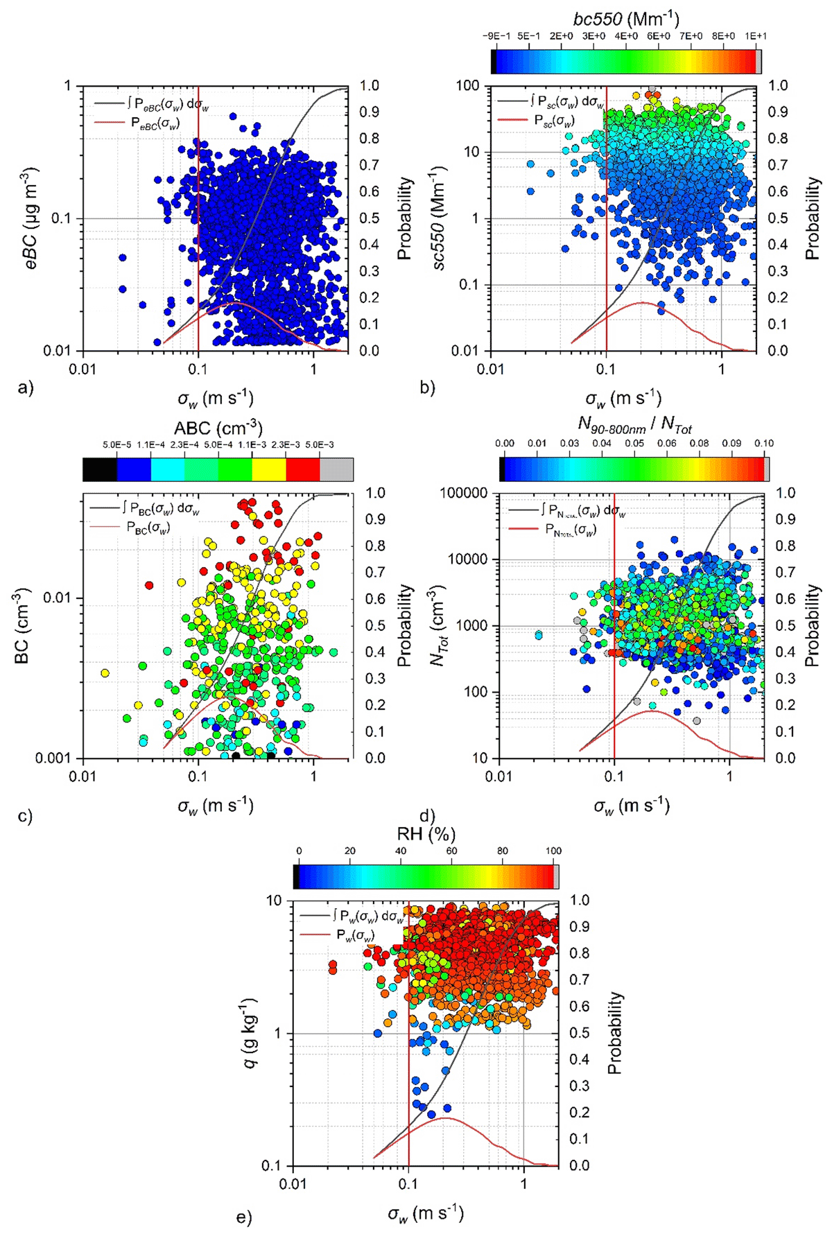
Figure 3
Scatter plots corresponding to a) eBC (μg m–3), b) sc550 and bc550 (Mm–1), c) BC and ABC (cm–3), d) Ntot (cm–3) and N90–800 nm/Ntot and e) q (g kg–1) and RH (%) in respect of σw (m s–1) as measured by HALO at (HAC)2 between 18 October to 26 November 2021. The red lines represent the normalized frequency of each measurement (called “Probability”), while the black lines are the integral of the normalized frequency of measurement (from the smallest σw value up to the given σw). The vertical red lines correspond to the σw threshold value of 0.1 m s–1 which indicates the transition between the PBL to the FTL regimes.
Based on these findings we can, thus, conclude that when σw > 0.1 m s–1 and σw < 0.1 m s–1, then (HAC)2 is inside and outside the PBL, respectively, while, when σw = 0.10 ± 0.01 m s–1, the mountaintop site is within the PBL entrainment (transition) zone. Thus, the value of σw = 0.10 ± 0.01 m s–1 can be regarded as a threshold to determine when (HAC)2 resides within the PBL, the FTL, or within the PBL transition zone.
We also calculated the Mean Normalized Bias (MNB) of the PBLH values against those retrieved using a σw threshold value of 0.1 m s–1. The PBLH values are aggregated into five different height ranges, from 400 to 1400 m with a step of 200 m (c.f. Figure 4). When the threshold σw values range within 0.09–0.11 m s–1, the MNB-PBLH varies within ±5%, consistent with observations by Schween et al. (2014). However, we found that the bias of the estimated PBLH compared to the true one, increases with respect to height. Thus, when using a σw threshold value equal to 0.13 m s–1, in the case where the true PBLH is lower than 600 m, the bias of the estimated PBLH is <±5%, while in the case where the true PBLH is higher than 1200 m, results in > ± 10%. This bias is amplified up to 30% when using larger σw threshold values leading to a significant overestimation of the PBLH especially in the case of deep planetary boundary layers. In conclusion, the threshold values of σw ranging from 0.09 to 0.11 m s–1, leads to a retrieval of the PBLH with a bias of ±5%.
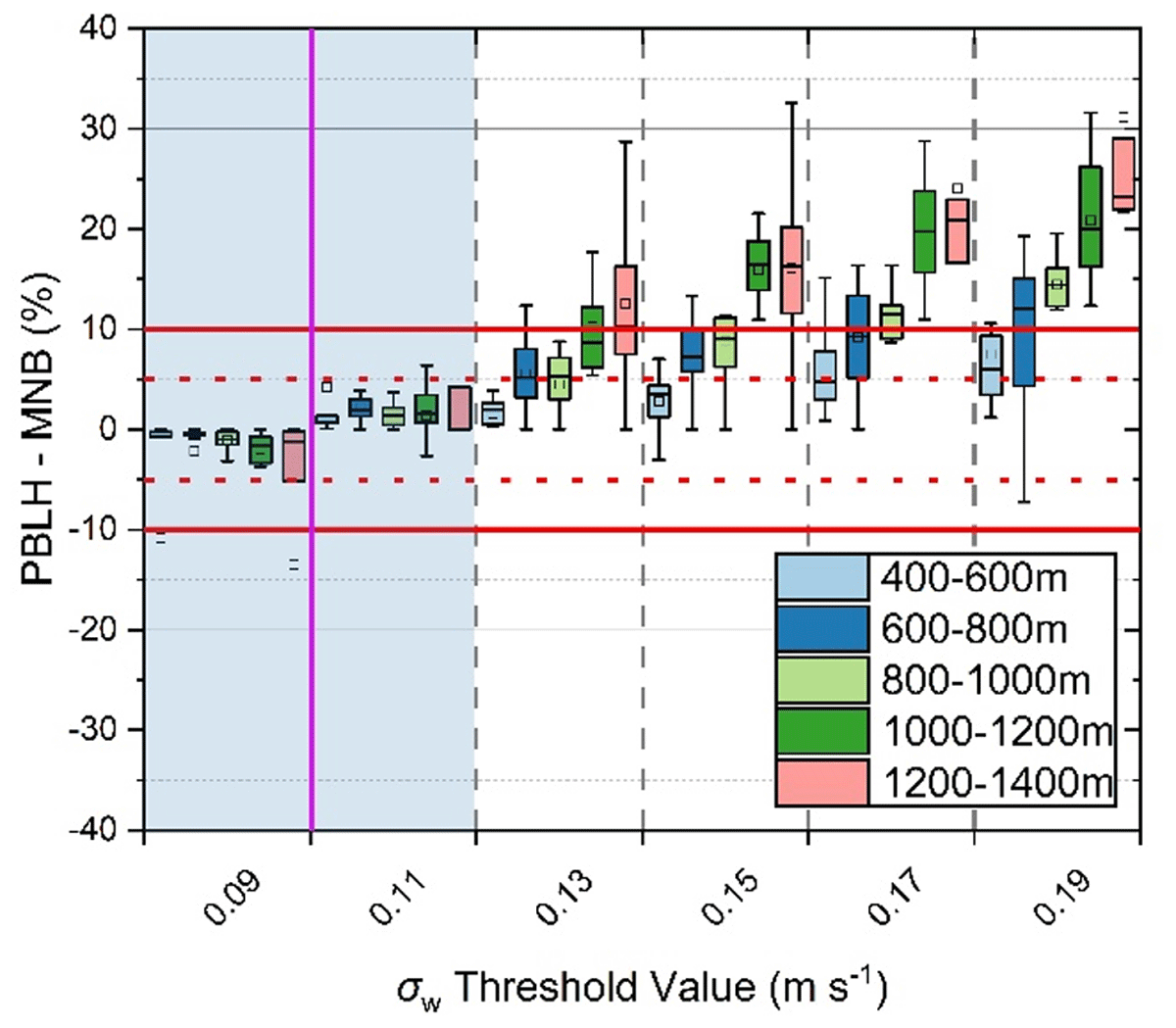
Figure 4
The PBLH-MNB (%) using σw threshold values 0.09 to 0.19 m s–1 compared to 0.1 m s–1 (magenta vertical line) at different PBLH ranges 400–600 m up to 1200–1400 m, respectively, between 18 October to 26 November 2021. The horizontal red solid and dashed lines correspond to a bias of ±5% and ±10%, while the shadow area depicts the σw threshold values where the MNB-PBLH (%) remains within ±15%.
3.2 Diurnal Evolution of the PBLH, AE31, WIBS and SMPS data
In this section, we aim to test the reliability of the threshold of σw of 0.1 m s–1 based on the diurnal evolution of the in situ measurements. The air masses and their corresponding diurnal cycles are distinctly different in load inside and outside the PBL. Therefore, we split the whole dataset into three subsets (c.f. Figure 5) based on the position of the (HAC)2 station compared to PBLH (retrieved using a σw = 0.1 m s–1), being the days where the PBLH:
exceeds the (HAC)2 altitude throughout the entire day, which occurs for 14 days (15–16, 18, 26, 30–31 October 2021; 5–7, 9 and 15–18 November 2021),
alternates above and below the (HAC)2 height during the day, which occurs for 24 days in the dataset (13–14, 17, 19, 20–23, and 27–29 October 2021; 1–4, 8, 10, 12–14, 19–21 and 23 November 2021),
remains below the (HAC)2 altitude throughout the entire day, which occurs for 3 days in the dataset (11, 22 and 24 November 2021).
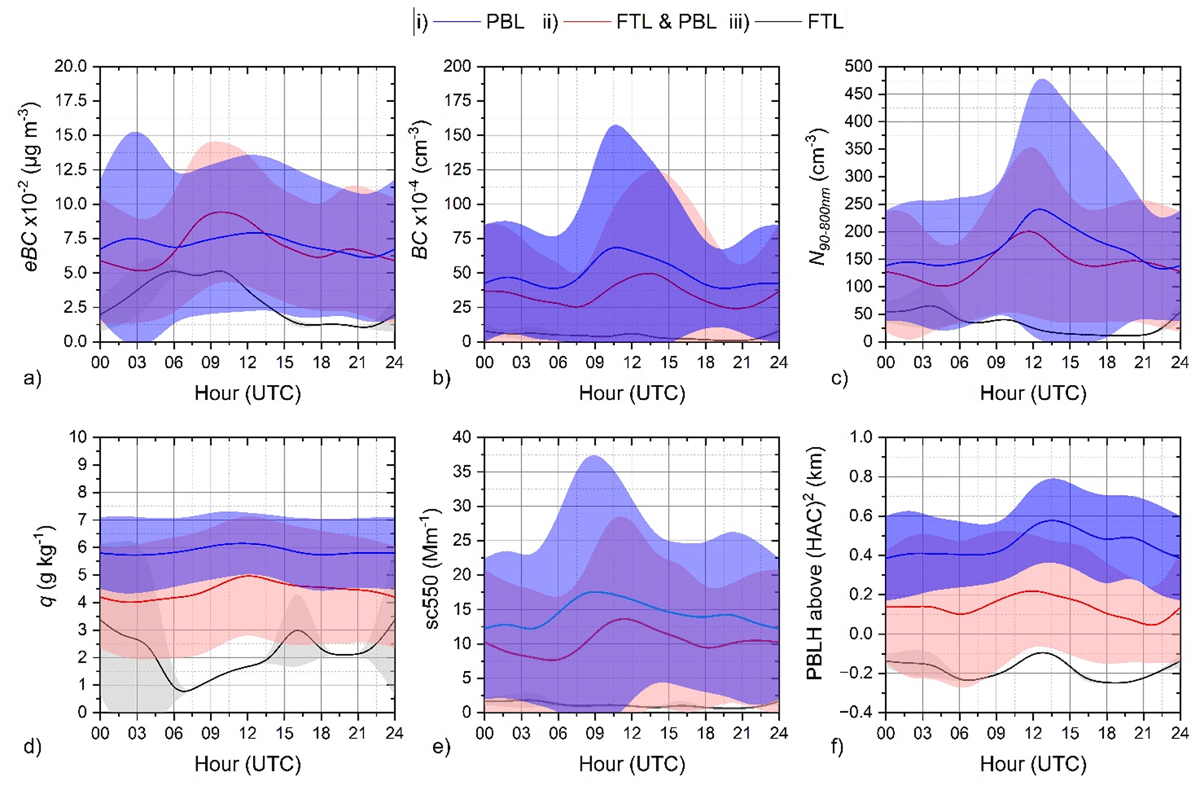
Figure 5
The diurnal cycle of a) eBC, b) BC, c) N90-800 nm, d) q, e) sc550 and f) PBLH for the three different subsets when (HAC)2 i) is within the PBL throughout the day (blue), ii) switches between the FTL and the PBL during the day (red), and iii) is within the FTL the entire day (black), between 18 October to 26 November 2021.
We found that when (HAC)2 is within the FTL, the aerosol and bioaerosol concentrations do not show a distinct diurnal cycle and are related to dry air masses (c.f. Figure 5), as all the in situ measured parameters have significantly lower values compared to the other subsets. Furthermore, a distinct diurnal cycle of eBC, BC, N90–800 nm, q, sc550 was also observed in subsets (i) and (ii), where (HAC)2 is either within the PBL throughout or part of the day (e.g. usually between 06:00–18:00 UTC about 60% of the days as shown in Figure 5 a) and b), as well as largest variations for the subset (i) which corresponds to the highest PBLH value.
Additionally, we calculated the mean diurnal variability of the PBLH for each month of the CALISHTO campaign (September 2021 to March 2022) (c.f. Figure 6), as well as the relative frequency of each subset (c.f. Figure 7a), and related them to three climatological regimes (Kallos et al.,1993), as follows: dry summer months (June–September), rainy winter months (November–February), and spring and autumn months (March–May and October), the latter are characterized by a transient season where the summer- and winter-type of weather patterns are interchanging.
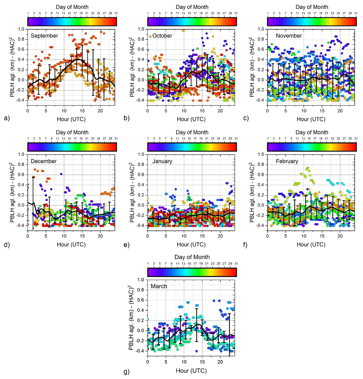
Figure 6
The monthly average diurnal cycle of PBLH for a) September 2021 up to g) March 2022. The PBLH values are colored by the day of the month. The solid black line corresponds to the hourly averaged values of the PBLH, while the error bars are the standard deviation of the PBLH values of each month, respectively.
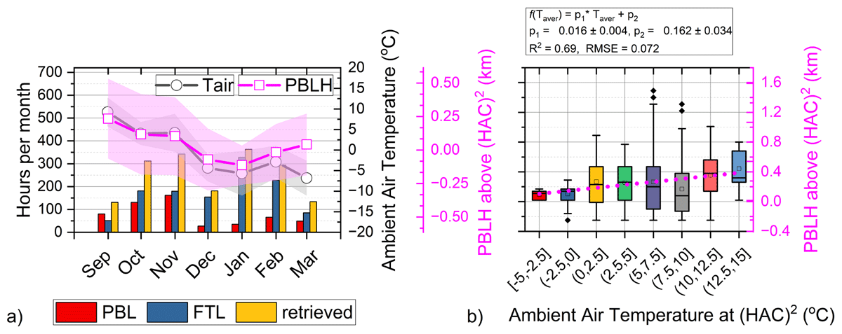
Figure 7
a) The histogram of the total hours where the (HAC)2 was within the PBL or FTL, and the seasonal trend of PBLH and the ambient air temperature, respectively; b) Boxplots of the PBLH values under cloud-free conditions based on the ambient air temperature at (HAC)2, grouped in bins from –5 up to 15°C with a step of 2.5°C, while the magenta dot line shows a linear relation between the ambient air temperature and the PBLH (September 2021 to March 2022).
In Figure 6 we can distinguish a seasonal cycle of the PBLH throughout the different seasons; thus, the maximum averaged PBLH is found during summer, while during November the PBLH values showed the largest variability compared to the other months. This is because November is characterized by frequent surface cyclonic systems over the greater Greek area, accompanied by a cold and a warm front moving westerly across Greece (Kouroutzoglou et al., 2011). As a result, (HAC)2 alternates between a cold and a warm domain of the barometric system, with important impacts on the PBLH: varying between 0 and 400 m above (HAC)2 for the first half of November, and 200 to 400 m below (HAC)2 level for the second half of the month. During the subsequent months, the PBLH and its variability decrease gradually until January, while later it increases steadily up to March. The average maximum values of the PBLH with respect to the (HAC)2 level per month were found equal to +400 m, +200 m, +50 m, –10 m, and –200 m, for September up to January, respectively.
Moreover, we calculated the total hours where the (HAC)2 is within the FTL or PBL per month, only under cloud-free conditions (c.f. Figure 7a). We found that in March and from September to November, the (HAC)2 alternates most of the time between the FTL and PBL, residing about half of the time within each layer. In contrast, between December and February (HAC)2 resides mostly within the FTL (around 85% of the time in average).
Finally, we grouped the dataset into nine groups (from –5o to 15°C with a step of 2.5°C), and we examined how PBLH varies with respect to the averaged ambient temperature at (HAC)2 level (c.f. Figure 7b). Thus, we calculated the mean PBLH value for each temperature range separately, and we interpolated a linear function between them. This interpolation (with R2 = 0.81) revealed that a 1°C increase in the surface mean temperature corresponds to a 16 ± 4 m increase of the averaged PBLH. This is a significant finding which offers valuable input data to climate models applied at high-altitude stations in the Mediterranean region, in connection to Global Warning scenarios.
4. Conclusions
In this paper we studied the variation of the PBL top-height in the vicinity of the (HAC)2 station at Mount Helmos, Greece. The identification of the PBLH was based on a synergy of data from a wind Doppler lidar and in situ instrumentation at the (HAC)2 station. The lidar was used to measure the vertical velocity of air masses and calculate the standard deviation of the updraft currents as an indicator of the vertical mixing in the PBL; the PBLH then corresponds to the height where the vertical velocity variability drops below a threshold that corresponds to when in-situ data determine when the (HAC)2 is at the PBLH. The in situ aerosol data obtained from a set of instruments (Aethalometer, Nephelometer, WIBS-5/NEO, SMPS), and data from a meteorological station, were used to determine the characteristics of the aerosols sampled, when (HAC)2 was within the PBL or in the FTL, respectively. We found that during daytime when (HAC)2 is within the PBL, the in situ sampled air masses are characterized by increased aerosol concentrations and increased humidity, while when (HAC)2 is within the FTL, the sampled air masses are characterized by low aerosol/bioaerosol concentrations and relatively low humidity. Therefore, given that these air masses are distinctly different in terms of their aerosol load and humidity inside or outside the PBL, showing intense diurnal cycles, we concluded that a threshold value of σw = 0.10 ± 0.01 m s–1 can be used to identify the PBLH at the (HAC)2 site and, thus, discriminate the transition zone between the PBL and the FTL.
We also examined the diurnal cycle of PBLH throughout the studied period and found that higher PBLH values are observed in September (400 m above (HAC)2), followed by a transition period in November, while the lower ones (200 m below (HAC)2) are observed during winter (December to February). The average maximum values of the PBLH with respect to the (HAC)2 level per month, ranged from +400 m down to –200 m (relative to to the (HAC)2 altitude), from September to January, respectively. It is important to mention that in March and from September to November, the (HAC)2 alternates most of the time between the FTL and PBL, residing about half of the time within each layer. In contrast, between December and February, (HAC)2 resides mostly within the FTL. A positive correlation between the mean ambient air temperature at (HAC)2 and mean PBLH was seen, corresponding to an PBLH increase of 16 m per 1°C increase of the surface temperature at (HAC)2 – which can be a useful constraint for atmospheric boundary layer dynamics in mountainous environments. Our methodology described here can be implemented to identify the origin of aerosols that feed orographic clouds and thus, potentially facilitating the retrieval of key cloud formation parameters and better understand aerosol-cloud-precipitation interactions in orographic clouds.
Acknowledgements
We also acknowledge support by the funding sources outlined below and by the Laboratory of Atmospheric Sciences and their Impacts (LAPI) of the École Polytechnique Fédérale de Lausanne, Switzerland and the Foundation for Research and Technology, Hellas.
Funding Information
This research was funded by the General Secretariat of Research and Innovation 105658/17-10-2019 in the framework of support of the research program “National Research Network for climate change and its effects” E.E –12365”, with Dr. K. Eleftheriadis as scientific coordinator. Part of this work was financed by the Basic Research Program PEVE (NTUA) under contract PEVE0011/2021. This work was supported by: PyroTRACH (ERC-2016-COG) funded from H2020-EU.1.1. (ERC), project ID 726165, the European Union’s Horizon Europe project “CleanCloud” (Grant agreement No. 101137639), and the “PANhellnfrastructure for Atmospheric Composition and climatE change” (MIS 5021516).
Competing Interests
The authors have no competing interests to declare.
Author Contributions
Conceptualization, R.F., K.E.; methodology, R.F., K.E., and P.K.; data analysis, R.F., M.I.G., E.D, S.V., K.G., and V.V.; model simulations, RF; investigation R.F., A.P., P.K, A.N.; writing—original draft preparation, R.F., K.E., A.P., P.K, A.N. and K.G.; review and editing, R.F., A.N., A.P., E.D, K.E., M.K., K.G., and V.V.; visualization, R.F.; supervision, R.F., K.E., A.P., A.N. and P.K.; All authors have read and agreed to the published version of the manuscript.