
Table 1
Comparison of the different verification metrics: ensemble spread vs ensemble spread (with and without observation errors), Dawid-Sebastiani score, and filter likelihood score. (y–z̄)2 is the squared error of the ensemble mean, the ensemble variance, and the error variance of the observations.
| VERIFICATION METRIC | EQUATION |
|---|---|
| RMSE | |
| RMSE w/obs | |
| DSS | |
| FLS |
Table 2
Radiosonde measured quantities and the (averaged) corresponding observation errors at different pressure levels.
| OBSERVED QUANTITY | PRESSURE LEVEL (HPA) | OBSERVATION ERROR |
|---|---|---|
| T | 200 | 0.83 K |
| T | 500 | 0.66 K |
| T | 850 | 0.90 K |
| u,v | 200 | 2.25 ms–1 |
| u,v | 500 | 1.89 ms–1 |
| u,v | 850 | 1.62 ms–1 |
| q | 500 | 0.000 38 kgkg–1 |
| q | 850 | 0.001 0 kgkg–1 |
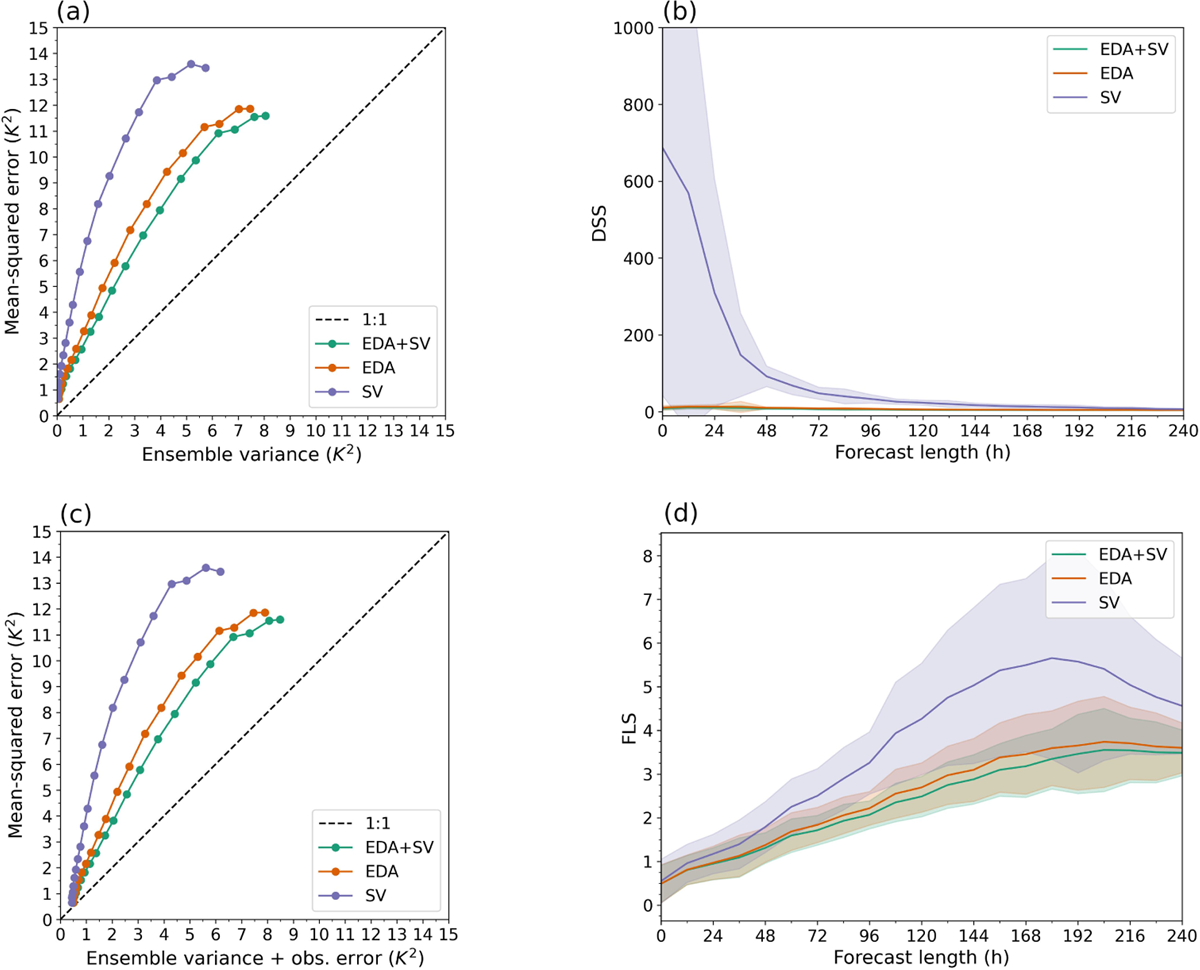
Figure 1
Different verification metrics for T500 in NH. Comparison between different verification metrics for temperature at 500 hPa in the Northern Hemisphere: (a) Ensemble spread-skill relationship, (b) Dawid-Sebastiani score, (c) Ensemble spread-skill relationship with observation error, and (d) Filter likelihood score. The solid lines show the mean value of the metric and the shaded area one standard deviation uncertainty. The green lines show forecasts with EDA and SV initial conditions, orange with EDA, and purple with SV. The dots in panels (a) and (c) show the spread (+obs.error)/error relationship for different forecast lead times every 12h.
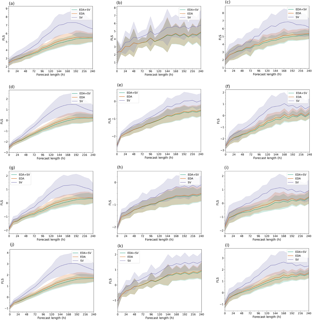
Figure 2
Combined FLS for different pressure levels. Sum of different variables for three different parts of the atmosphere, where the first row (a, b, c) shows temperature and horizontal wind components at 200 hPa, second row (d, e, f) shows temperature, horizontal wind components, and specific humidity at 500 hPa, third row (g, h, i) shows temperature, horizontal wind components, and specific humidity at 850 hPa, and the fourth row (j, k, l) the sum of above mentioned variables. The first column shows the results for the Northern Hemisphere, the second column for the Tropics, and the third column for the Southern Hemisphere. The green line shows EDA+SV, the orange EDA, and the purple SV. The solid line shows the mean value and the shaded area one standard deviation uncertainty.
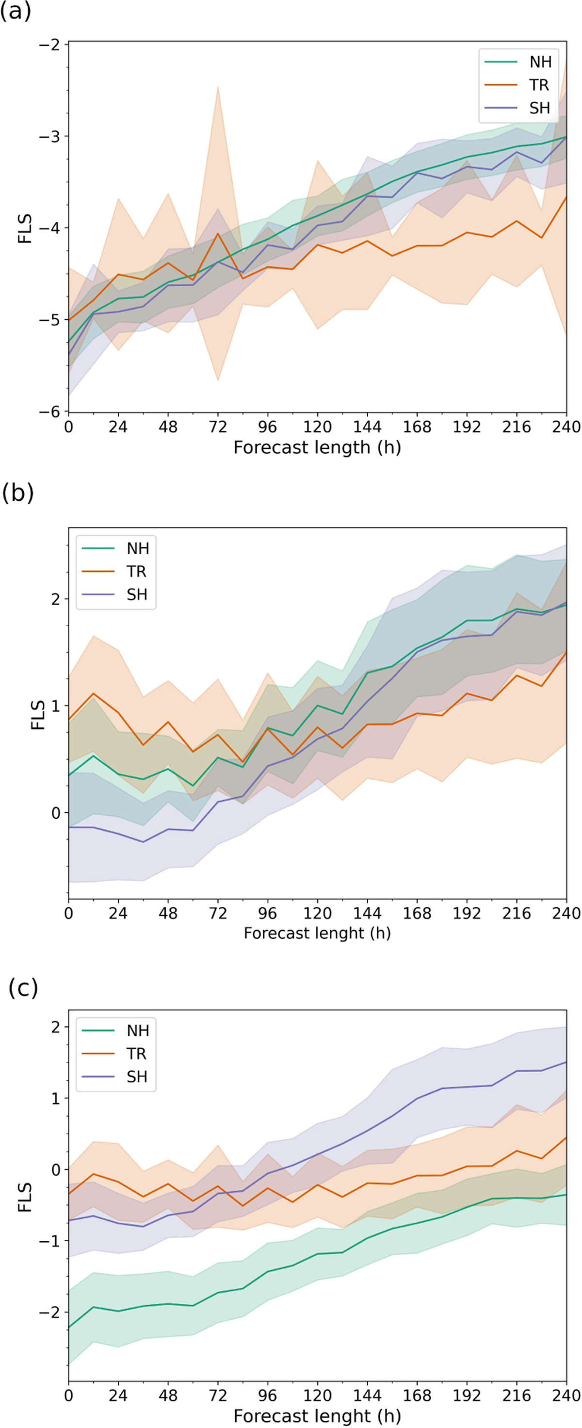
Figure 3
FLS for both satellite and sounding observations (a) Only sounding data, (b) Only satellite data, and (c) Combination of sounding and satellite data. Sum of different observation types: AMSU-A ch.5 brightness temperature and temperature at 200 hPa, 500 hPa, 850 hPa, and specific humidity at 500 hPa and 850 hPa for the ensemble system: EDA+SV+SPPT. The solid line shows the mean value over 53 ensemble forecasts and the shaded area one standard deviation uncertainty level for three different areas: green for the Northern hemisphere, orange for the Tropics, and purple for the Southern Hemisphere.
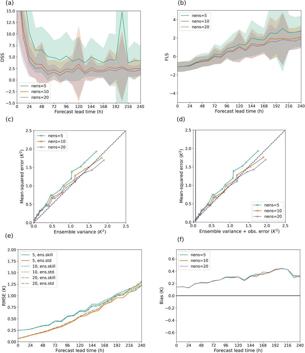
Figure 4
Verification metrics for different ensemble sizes (5, 10, and 20 members): (a) Dawid-Sebastiani score, (b) Filter likelihood score, (c) ensemble skill vs ensemble spread, (d) ensemble skill vs ensemble spread+observation error, (e) RMS error vs standard deviation of ensemble, and (f) Bias. Note that the vertical line in panel (d) marks the observation error. The data come from satellite METOP-A and the region is the Northern Hemisphere. The plots show verification metrics averaged over 53 ensemble forecasts initialised 7 days apart over one year.
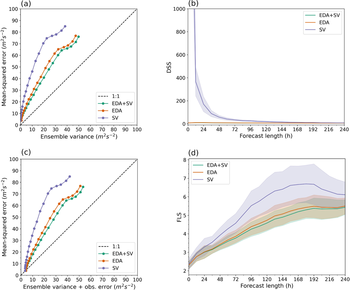
Figure 5
Different verification metrics for u500 in NH. Comparison between different verification metrics for wind component u at 500 hPa in the Northern Hemisphere: (a) Ensemble spread-skill relationship, (b) Dawid-Sebastiani score, (c) Ensemble spread-skill relationship with observation error, and (d) Filter likelihood score. The solid lines show the mean value of the metric and the shaded area one standard deviation uncertainty. The green line shows forecasts with EDA and SV initial conditions, orange with EDA, and purple with SV. The dots in panels (a) and (c) show the spread (+obs.error)/error relationship for different forecast lead times every 12h.
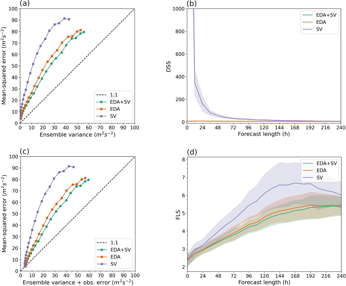
Figure 6
Different verification metrics for v500 in NH. Comparison between different verification metrics for wind component v at 500 hPa in the Northern Hemisphere: (a) Ensemble spread-skill relationship, (b) Dawid-Sebastiani score, (c) Ensemble spread-skill relationship with observation error, and (d) Filter likelihood score. The solid lines show the mean value of the metric and the shaded area one standard deviation uncertainty. The green line shows forecasts with EDA and SV initial conditions, orange with EDA, and purple with SV. The dots in panels (a) and (c) show the spread (+obs.error)/error relationship for different forecast lead times every 12h.
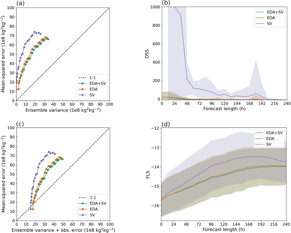
Figure 7
Different verification metrics for q500 in NH. Comparison between different verification metrics for specific humidity q at 500 hPa in the Northern Hemisphere: (a) Ensemble spread-skill relationship, (b) Dawid-Sebastiani score, (c) Ensemble spread-skill relationship with observation error, and (d) Filter likelihood score. The solid lines show the mean value of the metric and the shaded area one standard deviation uncertainty. The green line shows forecasts with EDA and SV initial conditions, orange with EDA, and purple with SV. Please note that in panel (a) and (c), the values are multiplied by 108. The dots in panels (a) and (c) show the spread (+obs.error)/error relationship for different forecast lead times every 12h.
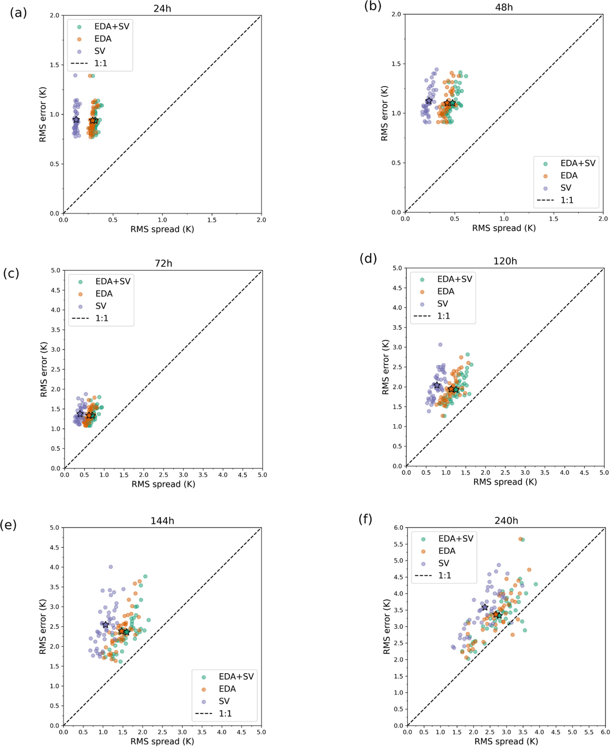
Figure 8
Root-mean squared (RMS) error versus spread for temperature at 500 hPa at different forecast lead times (a) 24h, (b) 48h, (c) 72h, (d) 120h, (e) 144h, and (f) 240h. One dot represents the RMS error/spread relationship for one ensemble forecast and the star is the mean over all ensembles. Green shows EDA+SV ensembles, orange EDA ensembles, and purple SV ensembles. The mean RMS error/spread relationship (marked with stars) corresponds to the dots in panel (a) of Figure 1.