
1. Introduction
Ensemble forecasting has been used for almost 30 years in numerical weather prediction to predict the flow-dependent forecast uncertainty (Buizza and Richardson 2017). In theory, the ensemble of forecasts should represent the true analysis error covariance at the initial time and the forecast error covariance during the time-evolution. Since these are unattainable in their full extent, some numerical approximations need to be applied (Leutbecher and Palmer 2008). At the European Centre for Medium-Range Weather Forecasts (ECMWF), for instance, initial value uncertainties are represented through a combination of Singular Vectors (SV) and Ensemble of Data Assimilations (EDA) (Buizza, Leutbecher, and Isaksen 2008; Isaksen et al. 2010) and the forecast model uncertainties with stochastic parametrisations (Leutbecher et al. 2017; Ollinaho et al. 2017). In fact, a host of approximations are available (Toth and Kalnay 1993, 1997; Houtekamer, Mitchell, and Deng 2009; Houtekamer et al. 2014; Bowler et al. 2008; Kay and Kim 2014; Miyoshi and Sato 2007; Zhang and Krishnamurti 1999; Wei et al. 2006, 2008; Christensen 2020; Buizza 2019). Modelling uncertainties can also be considered using, e.g., a multi-model ensemble or a perturbed parameter approach. Besides initial value perturbations and uncertainties of the model, also the horizontal and vertical resolution of the model, forecast length, and the number of ensemble members affect the reliability of an ensemble forecast (Buizza 2019). Since these methods provide approximations of the true uncertainties, it is important to assess how well they can reproduce the true flow-dependent forecast uncertainty.
An ensemble forecasting system is considered reliable when the skill of the ensemble mean and the spread of the ensemble members are equal (Leutbecher and Palmer 2008). This can be measured through different verification metrics by comparing the ensemble forecast against analyses or observations. Traditional approaches for verifying ensemble forecasts include the assessment of ensemble spread-error relationship (Leutbecher and Palmer 2008), rank histogram (Hamill 2001), and calculation of verification metrics such as continuous ranked probability score (CRPS, Hersbach 2000), and Dawid-Sebastiani score (the ignorance score for a Gaussian distribution, Dawid and Sebastiani 1999). These verification metrics do not directly account for errors of the observation or the analysis.
As weather prediction models improve and forecast errors gradually decrease, accounting for observational uncertainties in verification metrics becomes more important (see e.g., Ben Bouallegue et al. 2020; Ferro 2017; Duc and Saito 2018). Observation error in data assimilation is the sum of representativeness and instrumental errors, added with uncertainties from the observation operator. The observation error is estimated as a part of operational data assimilation and is therefore available for all observation types which are actively assimilated. Thus, a natural development step is to consider validation methods that account for observation errors.
Ferro (2017) considers proper scoring rules [scores that give honest results; the best forecast gets the lowest score (e.g., Gneiting and Raftery 2007)] for observation-based verification. Ferro (2017) introduces methods for forming error-corrected proper scoring rules that are insensitive to the quality of the observation for both categorical and numerical predictands. The author focuses on scoring rules for numerical predictands and takes Dawid-Sebastiani score as a starting point for these; one of these derived scores is a score referred to as the error-convolved logarithmic score. These error-corrected scores are only derived for univariate data, but a way of computing error-corrected scores for multivariate data is mentioned: computing the score for each observation followed by an average over the scores.
Yamaguchi et al. (2016) present a form of ensemble spread-error relationship where observation errors are included in the metric. They compare ensemble forecasts from ECMWF’s Integrated Forecasting System (IFS) against analyses, radiosonde observations, and satellite measurements for 1 day- and 5 day-forecasts. Inclusion of observation error makes the comparison of spread and error more realistic especially at short lead times where the observation error is large compared to the ensemble spread. They conclude that using observations in the validation of ensemble forecasts can give useful information about the system, and they also point out that estimating observation errors is important for obtaining reliable results.
Candille and Talagrand (2008) take a slightly different approach with a perturbed ensemble and introduce an approach called observational probability. The idea is to form an observation distribution with errors considered and compare the observation distribution against the distribution formed by the ensemble. In the perturbed ensemble approach random noise is added to the ensemble members to account for errors, a method presented in details by Saetra et al. (2004), which increases the spread of the ensemble.
Ben Bouallegue et al. (2020) focus on representativeness errors of SYNOP observations. They use the perturbed ensemble approach to account for uncertainties of observations and parametric models to form uncertainty distributions from which perturbations are drawn. The focus is on two metre air temperature, 10 metre wind speed, and daily precipitation.
Duc and Saito (2018) use Bayesian theory to form verification metrics that consider observation errors. They present a thorough background starting from the Bayes theorem before deriving the verification metrics based on likelihoods: the logarithmic score and its derived forms called weighted root-mean squared error (WRMSE) and Kullback-Leibler divergence. They use the log-likelihood metric for deterministic and ensemble forecasts for both univariate and multivariate data. As an application, WRMSE is used to analyse three different data assimilation techniques against radio soundings in a limited area around Japan.
The focus in this paper is on the filter likelihood score, a score similar to the ones described in (Duc and Saito 2018) and the error-convolved logarithmic score described in (Ferro 2017). As is later noted, the filter likelihood score could also be seen as a multi-dimensional extension of the error-convolved logarithmic score.
In Bayesian estimation, prior information is updated with measurements such that the uncertainty of the posterior estimate explicitly depends on the uncertainty of the prior information and measurements. In other words, the uncertainty of the forecast is estimated based on both the forecast itself and observations, once available. Since filter likelihood emerges from this principle, it naturally accounts for both forecast and observational uncertainties. In this study, we use OpenIFS-based ensemble forecasts and observations from radiosondes and satellites to pose the following questions:
Is filter likelihood score able to distinguish between different ensemble systems of a realistic model (i.e., is it sensitive enough to detect slight differences in initial state perturbations)?
Is it possible in practise to formulate a multivariate filter likelihood score with different observation types as an input?
How does a reduced ensemble size affect filter likelihood score?
In previous studies, filter likelihood has been used as a cost function for optimisation of parameters in idealised set-ups with the Lorenz’95 model (Hakkarainen et al. 2012, 2013; Solonen and Järvinen 2013; Ekblom et al. 2020). Hakkarainen et al. (2012) study three different methods for estimating closure parameters in a Lorenz’95 system, and one of these methods is the filter likelihood approach. Hakkarainen et al. (2013) use filter likelihood from extended Kalman filter and ensemble adjustment Kalman filter for tuning closure parameters of a Lorenz’95 system using a Markov chain Monte Carlo method. Solonen and Järvinen (2013) demonstrate with Lorenz’95 model how filter likelihood can be used as an approach for tuning an ensemble prediction system by showing a link between the filter likelihood and traditional verification metrics (rank histogram, continuous ranked probability score, and ensemble spread-error relationship).
This paper extends the use of filter likelihood to realistic models and observations with the following outline. Section 2 presents the theory behind filter likelihood score (FLS) and Section 3 compares FLS to traditional verification metrics, Section 4 introduces the forecast data and observations used, and Section 5 presents the results. Sections 6 and 7 discuss and conclude the study.
2. Filter Likelihood Score
In this section, we present the theory of filter likelihood score and derive the equation for the verification metric.
2.1. Filter likelihood score (FLS)
We are interested in knowing how good forecasts a model produces when comparing the forecasts against observations. For an optimal forecast system, the forecast distribution reflects the actual forecast uncertainty (Gneiting, Balabdaoui, and Raftery 2007). We assume that a forecast system produces probabilistic forecasts from a forecast distribution depending on the model. This is denoted as , where z = {z1, … zN} is an ensemble with N independently sampled members from the forecast distribution and the model. In addition, we assume that this ensemble has already been mapped to the observation space by an observation operator as , where x is the raw forecast representing the discrete model variables. Hence, the ensemble forecast z can be directly compared to the observation vector y. The dimension of the raw forecast x depends on the resolution of the model and the number of forecast variables. The dimensions of z and y depend on how many variables we observe and over how many spatial and temporal locations.
Observational uncertainty arises from the representativeness of observations and uncertainties both in the measurements and the operator and this uncertainty is covered by the observation distribution p(y | z). The likelihood for observing y given the model can be calculated by averaging over the forecast uncertainty
As in Duc and Saito (2018), this can be seen as observational evidence for the model and be used as a score. The forecast ensemble as a sample from can be used to evaluate the integral in (1).
For a perfect forecast system and with Gaussian observation uncertainty, we have , where Σy is the observation uncertainty covariance matrix, which is typically assumed diagonal. If, also, the forecast distribution can be approximated by a Gaussian distribution (or by the first two moments) we have , with ensemble mean z̄ and ensemble covariance matrix Σz as estimates for the forecast mean μ and the forecast uncertainty covariance C. The covariance is calculated between the forecast variables in each ensemble member, and in principle also between different forecast locations and times within the ensemble. In the applications, we will be using ensemble standard deviations, only.
Assuming Gaussianity, the ensemble provides an approximation of the evidence (1) as
which, when written as minus twice the logarithm of the likelihood, becomes
In the equation above we have omitted the terms that do not depend on the model, but only on the correct probability scaling of the likelihood density. Equation (3) can be seen as the ignorance score for a Gaussian ensemble system that acknowledges the observation uncertainty (Siegert et al. 2019). We will call it filter likelihood score (FLS) as it can be directly motivated by considering the ensemble prediction system as an ensemble data assimilation system, which in turn connects the score to Kalman filter likelihood. This motivation is explained in more detail in Appendix A.
As with any ensemble system, the estimation of covariance matrices from ensembles with limited size will lead to spurious correlations between far away points in the state space and this calls for some kind of regularisation in a form of variance localisation. The simplest way is to assume all mutual correlations to vanish and use only the diagonal elements of the covariances. The univariate filter likelihood score is formed from individual ensemble standard deviations σz,i for the each observed quantity i and the observation uncertainty σo,i:
where the z̄i is the ensemble mean, σz,i is the ensemble standard deviation, σo,i is the observation uncertainty standard deviation for yi, for variable i, and summation is over the L observations. Equation (4) is adopted from (Hakkarainen et al. 2013), but here we divide by the number of observations to assure comparability when the number of observations is not constant. Note that when equation (4) is multiplied by 2 and the number of observations is 1 (L = 1), the equation is the same as the error-convolved logarithmic score presented by Ferro (2017). The error-convolved logarithmic score is proper under the assumption of the white noise model, but is sensitive to the quality of observations.
A multivariate version of the score from equation (3) would be used, for example, when we want to account for the between variable correlation at the observing locations. We then have
where for each multivariate observation yi we calculate the corresponding ensemble covariance Σz,i = cov(zi) and Σy,i is the observation uncertainty covariance for yi. When assuming zero correlation between the variables the combined score will be equal to the univariate score in equation (4) when, in addition, summation is done over each of the variables.
3. Verification Metrics for Ensemble Prediction
This section presents the different verification metrics used for comparing the filter likelihood score.
3.1. Ensemble spread-error relationship
An ensemble forecast system is considered reliable when the relationship between the ensemble error and the ensemble spread is, on average, equal (Leutbecher and Palmer 2008). This can be formulated as
where M is the number of ensemble forecasts, N the size of the ensemble, ϵ = y–z is the ensemble mean error (deviation of the ensemble mean from observation, truth, or analysis) and σz is the spread of the ensemble members around the ensemble mean (and its square the variance of the ensemble).
3.2. Ensemble spread-error with observation errors considered
The original ensemble spread-error relationship does not consider any observational or analysis errors. Yamaguchi et al. (2016) derive a formula of the ensemble spread-error relationship, where observation errors are included. In this error-corrected ensemble spread-error relationship, the ensemble mean skill should be in balance with the sum of ensemble spread and observation error (Yamaguchi et al. 2016, Eq. 7):
where σo is the observation error.
3.3. Dawid-Sebastiani score (DSS)
Dawid-Sebastiani score (DSS, Dawid and Sebastiani 1999) comes from the ignorance score of a Gaussian distribution with ensemble mean z̄ and ensemble standard deviation spread σz. In the univariate case it takes the form (eq. 6.10, Vannitsem, Wilks, and Messner 2018)
and in the multivariate case (eq. 6.24, Vannitsem, Wilks, and Messner 2018)
where y is the vector of observed values, z̄ is the ensemble mean vector, and Σz is the covariance matrix of the ensemble.
If we ignore the correlations between observations in the ensemble, then Σz is a diagonal matrix and, similarly as for FLS, we can then approximate the DSS score with
where L is the number of observations, yi the observed value, z̄i is the ensemble mean, and σz,i the ensemble spread corresponding to observation i. Similarly as for FLS, we divide equation (10) by the number of observations L. This assures comparability when the number of observations varies.
Table 1 summarises the verification metrics used in this study. The table shows the similarities between the different metrics: the ensemble mean skill and the ensemble error are both present in all verification metrics. The filter likelihood score and the ensemble spread-error relationship with observation errors also consider observation error in the calculations. Dawid-Sebastiani score is a special case of the filter likelihood score for cases where observation errors are zero. As is later seen, due to the absence of observational errors in DSS its behaviour can be quite different compared to FLS.
Table 1
Comparison of the different verification metrics: ensemble spread vs ensemble spread (with and without observation errors), Dawid-Sebastiani score, and filter likelihood score. (y–z̄)2 is the squared error of the ensemble mean, the ensemble variance, and the error variance of the observations.
| VERIFICATION METRIC | EQUATION |
|---|---|
| RMSE | |
| RMSE w/obs | |
| DSS | |
| FLS |
4. Forecast Data and Observations
In this section, we describe the ensemble forecast data and observational data used in the verification metrics.
4.1. OpenIFS ensemble forecasts
The ECMWF OpenIFS model is a portable version of the ECMWF’s operationally active NWP model. OpenIFS is available upon registration to ECMWF member state hydro-meteorological services, universities, and research institutes for research and education purposes, and can be used in a variety of hardware setups. The OpenIFS model provides to the users in essence the same top-of-the-line NWP forecast model as the operational model. The key differences between the two models are: OpenIFS does not include the data-assimilation codes or capabilities of IFS, and the latest release version of OpenIFS is based on the IFS version operational between 2017–2018 (CY43R3), for more details see e.g. Ollinaho et al. (2021).
In this study, data from two different OpenIFS ensemble runs is used:
OpenIFS version CY40R1 is here used to run 20 member ensembles with horizontal resolution of ∼32 km (TL639). We use this setup to run 10-day atmospheric forecasts for three different types of initial state perturbations: EDA only, SV only, and combined EDA and SV. We refer an interested reader to Ollinaho et al. (2021) for more details about the initial state perturbations. In total 44 ensembles are launched 8 days apart for dates between December 1st 2016 and November 18th 2017. This ensemble set is used to compare different verification metrics and in calculating the filter likelihood score against sounding data.
OpenIFS version CY40R1v1 is used here with the same ensemble size and resolution as in (1) launched every 7 days apart between December 1st 2016 and November 30th 2017 resulting in a total of 53 ensembles. The ensemble here is launched with EDA and SV perturbations in the initial states and with a stochastic model uncertainty component active in all model forecasts (SPPT). This ensemble is used to calculate filter likelihood against AMSU-A channel 5 data.
We will refer to these data sets as data set (1) and (2). The reason behind the two different ensemble sets lies in the observation operator for the satellite observations. The observation operator requires many model output fields, which were not available through the original ensemble sets. Due to computational resources we only included one ensemble set for the satellite observations.
The scores are calculated separately for each forecast lead time (or over a time window for the satellite data) at 12-h interval up to 240 hours. The resulting values are further averaged over different observation locations (or the three geographical regions for the soundings) and the 44 and 53 ensemble runs in data set (1) and (2), respectively.
4.2. Observations
In this study, we look at two types of observations: radio soundings and satellite data. The radio soundings are global TEMP observations launched at 00UTC and 12UTC. The satellite data are measurements from AMSU-A channel 5 at observation times of 00UTC and 12UTC.
4.2.1. Radiosondes
Radiosondes measure temperature, specific humidity, and horizontal wind components at different levels of the atmosphere. In this study, we use global radiosondes launched at 00UTC and 12UTC between 1 December 2016 and 30 November 2017. The radiosondes including observation errors are downloaded from ECMWF’s Meteorological Archival and Retrieval System (MARS).
The raw sounding data are interpolated in vertical direction and the horizontal position is kept constant. The vertical interpolation is computed in log(p) coordinate to given pressure levels: 200 hPa, 500 hPa, and 850 hPa. For simplicity, the location of the observation for all levels is the position of the launching area. We only interpolate the data; values out of range are set to NotANumber. The observation errors are interpolated in a similar manner as the observations. Table 2 shows the observed quantities and their corresponding observation errors used in this study. The errors are calculated as the mean over all interpolated data points and are thus not held constant. We do not include covariances in the calculation of the verification metrics.
Table 2
Radiosonde measured quantities and the (averaged) corresponding observation errors at different pressure levels.
| OBSERVED QUANTITY | PRESSURE LEVEL (HPA) | OBSERVATION ERROR |
|---|---|---|
| T | 200 | 0.83 K |
| T | 500 | 0.66 K |
| T | 850 | 0.90 K |
| u,v | 200 | 2.25 ms–1 |
| u,v | 500 | 1.89 ms–1 |
| u,v | 850 | 1.62 ms–1 |
| q | 500 | 0.000 38 kgkg–1 |
| q | 850 | 0.001 0 kgkg–1 |
When comparing the model data against the radio sounding data, the gridded model data are interpolated in the horizontal plane to the observation points using Scipy RegularGridInterpolator with linear interpolation (Virtanen et al. 2020). The verification metrics are then calculated in observation space. When computing the verification metrics, the data are divided into three regions: Northern Hemisphere (>20°N), Tropics (20°S–20°N), and Southern Hemisphere (>20°S). Note that the number of observations in the Tropics and the Southern Hemisphere is smaller than in the Northern Hemisphere. The total number of observations at one time instance are about 460–500 in the Northern Hemisphere, about 100 in the Tropics, and about 50 in the Southern Hemisphere.
4.2.2. Satellite data
Besides conventional radiosondes, we use Advanced Microwave Sounding Unit A (AMSU-A) channel 5 remote sensing observations. AMSU-A channel 5 consists of two frequency bands at 53.596 ± 0.115 GHz. AMSU-A channel 5 has been primarily designed to sound tropospheric temperature with a maximum of sensitivity at approximately 4 km altitude. However, AMSU-A channel 5 is also somewhat sensitive to tropospheric hydrometeors (e.g., cloud droplets and ice crystals) and surface temperature. The surface transmittance of AMSU-A channel 5 is about 12%. More details of AMSU-A channels can be found for example in Geer, Bauer, and English (2012) and Bormann and Bauer (2010).
The AMSU-A channel 5 data set covering 1 December 2016 to 10 December 2017 was retrieved from MARS. During the chosen time period AMSU-A instrument was active on five satellites: METOP-A, METOP-B, NOAA15, NOAA18, and NOAA19. For each day of the time period observations at 00UTC and 12UTC are selected with a cut-off time of ±30 minutes resulting in batches of 7000–8000 observations. Other cut-off times were also considered but ±30 min was chosen as a reasonable balance between selecting as many observations as possible and not deviating too much from the verification times. The observations are further corrected by subtracting the operational bias correction coefficients computed during the variational data assimilation. The bias correction intends to correct systematic biases caused by instrument calibration, satellite position drift, varying scan position, and other reasons (see, e.g. McNally 2006). We use the instrument and channel specific noise equivalent temperature (NET) as the observation error. NET represents how large brightness temperature variations are caused by internal noise of the instrument. For AMSU-A channel 5 NET is 0.25K (Geer Bauer, and English 2012).
Conversion of the model fields into brightness temperature in observation space is performed with Radiance Simulator software (NWP-SAF 2021). Radiance Simulator is a wrapper for the RTTOV library (Saunders et al. 2018) and uses the metadata associated with the observations to compute the model counterparts from the forecast fields of OpenIFS (see user guide of Radiance Simulator for details).
5. Results
The results are divided into four different subsections:
How the filter likelihood score compares with ensemble spread-error relationships and Dawid-Sebastiani score;
Combined filter likelihood score over several variables for different parts of the atmosphere and geographical regions;
How the filter likelihood score behaves when having two different types of observations;
How the filter likelihood score reacts on reduction of ensemble size,
where the first two use data set (1) and the last two use data set (2).
5.1. Comparisons between different verification metrics
In Figure 1, we compare verification metrics for temperature at 500 hPa from radio soundings and the three different ensemble systems: EDA+SV, EDA, and SV. The area is the Northern Hemisphere (>20°N; NH). Panel (a) shows the ensemble spread-error relationship, (b) Dawid-Sebastiani score, (c) ensemble spread-error relationship with observation errors, and (d) filter likelihood score. All verification metrics are computed as the mean over all ensemble forecasts (a total of 44 ensemble forecasts) with the shaded area showing one standard deviation uncertainty level.
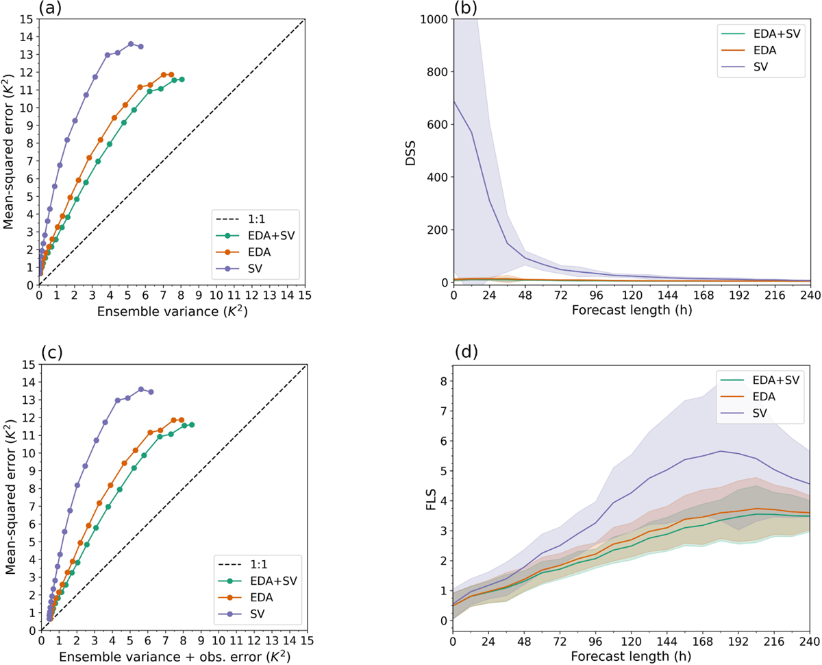
Figure 1
Different verification metrics for T500 in NH. Comparison between different verification metrics for temperature at 500 hPa in the Northern Hemisphere: (a) Ensemble spread-skill relationship, (b) Dawid-Sebastiani score, (c) Ensemble spread-skill relationship with observation error, and (d) Filter likelihood score. The solid lines show the mean value of the metric and the shaded area one standard deviation uncertainty. The green lines show forecasts with EDA and SV initial conditions, orange with EDA, and purple with SV. The dots in panels (a) and (c) show the spread (+obs.error)/error relationship for different forecast lead times every 12h.
When comparing the verification metrics in Figure 1, we note that the different ensemble systems are arranged in the same order for all four verification metrics. The system with EDA+SV (green) scores the best, followed closely by EDA (orange), and SV (purple) scores the worst. This shows that the filter likelihood score is consistent with traditional verification metrics (see e.g. Ollinaho et al. 2021) and is expected from previous studies with Lorenz’95 (Solonen and Järvinen 2013). Similar results are obtained for horizontal wind components u and v and specific humidity q (see Figures 5, 6 and 7 in the Appendix). Figure 8 in the Appendix shows a more detailed analysis of the RMS error/spread relationship for temperature at 500hPa. We note that the FLS is negative for specific humidity, a result of small values in the logarithm term. Still, the order of the ensemble systems stays the same – the system with SV clearly has the highest value and the difference between the other two systems is small with EDA+SV scoring the best.
5.2. Comparisons between different ensemble systems
Next, we will look at how well the filter likelihood score preserves the order of the ensemble system when a combined FLS of several radio sounding observations is formed. Figure 2 presents the results for the combined filter likelihood score at three different pressure levels as well as the sum of the variables at these three levels. Panels (a, b, c) show FLS for the combination of horizontal wind components u and v, and temperature T at 200 hPa for the Northern Hemisphere (NH), the Tropics (TR), and the Southern Hemisphere (SH). Panels (d, e, f) and (g, h, i) show for the same regions the combination of specific humidity, temperature, and horizontal wind components at 500 hPa and 850 hPa, respectively. Panels (j, k, l) show the sum of the above mentioned variables as one overall metric for the three regions NH, TR, and SH. All verification metrics are computed as the mean over all ensemble forecasts with the shaded area showing one standard deviation uncertainty level. The results show consistency of the order of the ensemble systems for the three regions. The difference between EDA+SV and EDA is small, especially for the tropical region, whereas SV clearly scores higher (worse). The figure shows that for a combined FLS of different variables for different parts of the atmosphere, the order of the ensemble system stays the same as for the univariate case (Figure 1). Note that when including specific humidity in the metric, FLS becomes negative. This happens when the values in the logarithm term of eq. 4 are smaller than 1 as is the case for specific humidity (cf. Table 2 and Figure 7). However, this does not affect the interpretation of the score.
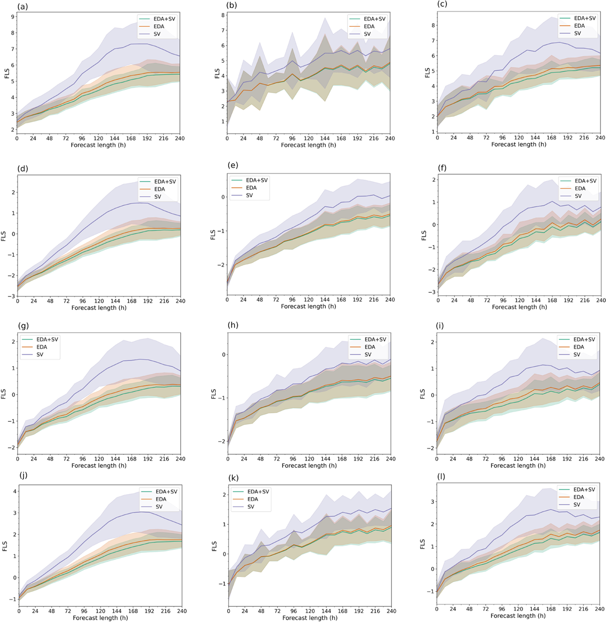
Figure 2
Combined FLS for different pressure levels. Sum of different variables for three different parts of the atmosphere, where the first row (a, b, c) shows temperature and horizontal wind components at 200 hPa, second row (d, e, f) shows temperature, horizontal wind components, and specific humidity at 500 hPa, third row (g, h, i) shows temperature, horizontal wind components, and specific humidity at 850 hPa, and the fourth row (j, k, l) the sum of above mentioned variables. The first column shows the results for the Northern Hemisphere, the second column for the Tropics, and the third column for the Southern Hemisphere. The green line shows EDA+SV, the orange EDA, and the purple SV. The solid line shows the mean value and the shaded area one standard deviation uncertainty.
In the tropics, there is larger variation in the upper atmosphere than in the mid and lower troposphere [compare panels (b, e, h) in Fig 2], visible from the larger shaded area. The reason behind this is unknown to us and needs further studying, but could be related to the tropopause or diurnal variations. In the Southern and Northern Hemisphere, this is also noted, but the difference is smaller. As there are more observations in the Northern Hemisphere than in the Tropics, we can expect a smoother result here. However, this is not the case for the Southern Hemisphere as there are fewer observations than in the Tropics. The mean value is quite smooth for all three regions at the three different pressure levels.
5.3. Filter likelihood with satellite data
Filter likelihood score shows consistency when comparing different ensemble systems for radio sounding measurements. From equation (4), we note that summation over different observation types is possible if we form a vector containing observations of several variables y = {y1, …, yL} as we can split the sum into several sub-sums, one for each observed quantity. Figure 3 looks at the combined filter likelihood score of satellite data and radiosonde measurements (temperature at 200 hPa, 500 hPa, 850 hPa, and specific humidity at 500 hPa and 850 hPa). The figure shows FLS for one ensemble system (EDA+SV with SPPT) for three different regions: Northern Hemisphere (green), Tropics (orange), and Southern Hemisphere (purple). In panel (a) and panel (b) the FLS is calculated for sounding data and satellite data only and in panel (c) FLS is calculated for the combination of sounding and satellite data. As FLS is weighted by the number of observations, we note that the total score in panel (c) for the Northern Hemisphere is pushed further down than the score for the Tropics and the Southern Hemisphere since there are more sounding observations in the NH area. Similarly, the total score is closer to the score with only satellite data than with only sounding data as more weight is put on the satellite data (higher number of observations). The filter likelihood score behaves as before; the shorter the forecast, the better (lower) the score. An exception is in the Tropics, where the FLS for satellite data first decreases with forecast lead time before starting to increase with lead time. We also note a steady increase of the (averaged) score with forecast range. The error (shaded area) does not seem to vary with forecast lead time. However, we did not compare different ensemble systems when including satellite data. Instead, we analysed the effect of ensemble size for one example satellite and region.
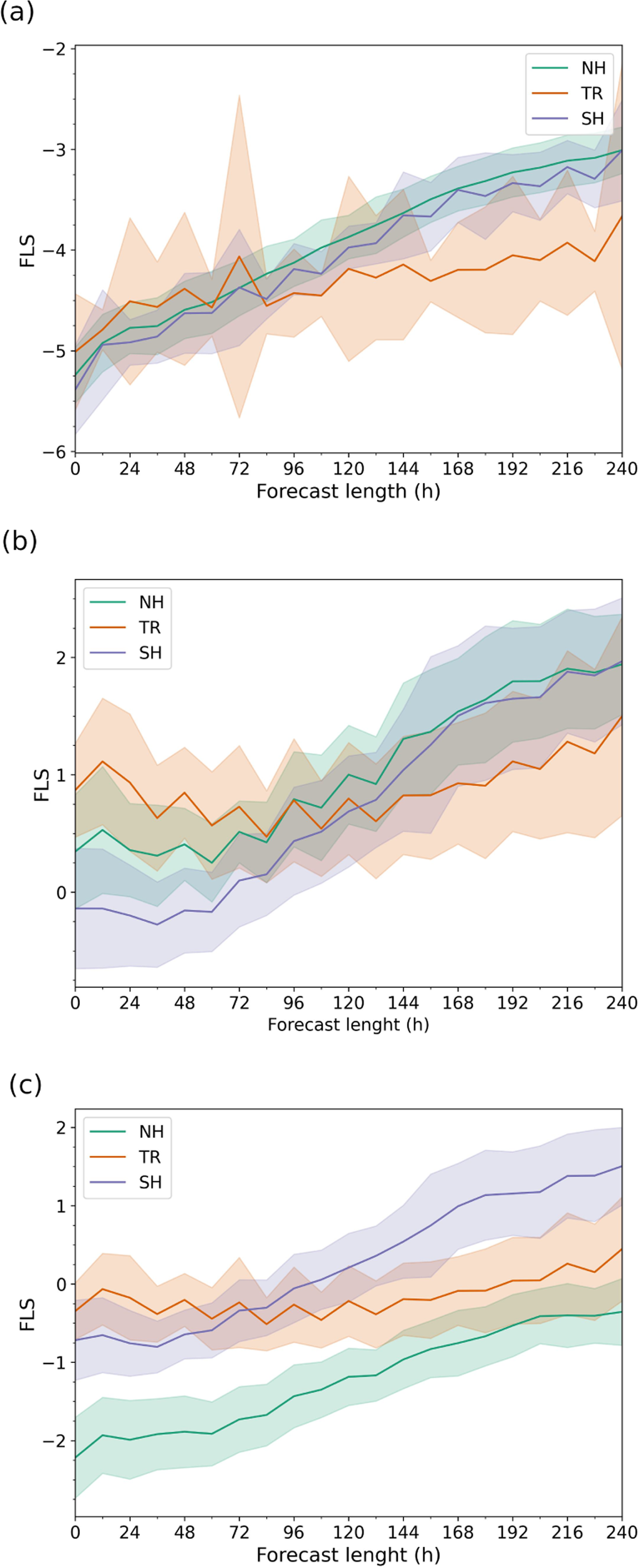
Figure 3
FLS for both satellite and sounding observations (a) Only sounding data, (b) Only satellite data, and (c) Combination of sounding and satellite data. Sum of different observation types: AMSU-A ch.5 brightness temperature and temperature at 200 hPa, 500 hPa, 850 hPa, and specific humidity at 500 hPa and 850 hPa for the ensemble system: EDA+SV+SPPT. The solid line shows the mean value over 53 ensemble forecasts and the shaded area one standard deviation uncertainty level for three different areas: green for the Northern hemisphere, orange for the Tropics, and purple for the Southern Hemisphere.
5.4. Satellite data: effect of reduced ensemble size
Figure 4 shows an example of how different verification metrics are affected when the ensemble size is reduced. We consider only one satellite (METOP-A) in the Northern Hemisphere and compare the different verification metrics for ensembles with 5, 10, and 20 members. Figure 4 shows that the larger the ensemble size, the better (smaller) the scores are. This applies to all verification metrics compared. However, the difference between an ensemble of 10 and 20 members is small. When looking at panel (e), we note that the ensemble skill (ensemble mean error) is almost the same for the three ensemble sizes at shorter lead times. At short lead times, the difference between the ensemble spread and the ensemble skill is larger than at longer lead times. We also note that when including observation error in the validation (panel (d)), the ensemble spread-error relationship is closer to the one-to-one line.
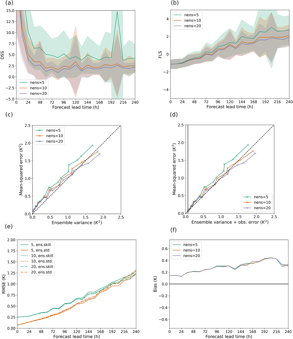
Figure 4
Verification metrics for different ensemble sizes (5, 10, and 20 members): (a) Dawid-Sebastiani score, (b) Filter likelihood score, (c) ensemble skill vs ensemble spread, (d) ensemble skill vs ensemble spread+observation error, (e) RMS error vs standard deviation of ensemble, and (f) Bias. Note that the vertical line in panel (d) marks the observation error. The data come from satellite METOP-A and the region is the Northern Hemisphere. The plots show verification metrics averaged over 53 ensemble forecasts initialised 7 days apart over one year.
Using different five-member subsets does not seem to change the results for the case of a five-member ensemble. Similarly, a different subset for the 10-member ensemble do not seem to change the results (not shown).
6. Discussion
From studies with the idealised model Lorenz’95, we know that filter likelihood score is consistent with traditional verification metrics and sensitive to different set-ups of the ensemble system (Solonen and Järvinen 2013). The results here show that this is the case also for a realistic NWP model. Moreover, it is possible to form a multivariate version of filter likelihood score, but here we did not use fully multivariate FLS as the covariance matrices were assumed diagonal. The filter likelihood score performs well for comparing different ensemble system set-ups for both uni- and multivariate data. Duc and Saito (2018) used a similar score with a different naming (weighted RMSE), but only for 12h forecasts and in a limited area. Here, we have shown that filter likelihood score also works for global data and different geographical regions, and longer range forecasts (up to 10 days). Furthermore, we looked at different observation types and combined radio soundings and satellite measurements into one combined score. However, if FLS is to be used as a stand alone verification metric, verifying the results together with other verification metrics might be useful for a complete picture. For example, the filter likelihood score does not directly tell whether the system is over- or underdispersive. For this, a rank histogram or a spread-skill relationship could be used in addition to FLS.
Filter likelihood score is not the only option for computing a combined score over different observations. As an example, it is possible to compute a combined CRPS over several quantities, but the data need to be normalised before combining it into a single score. Computing a combined CRPS with normalised data of temperature, wind components, and specific humidity at 500hPa gives similar results with the ensemble systems appearing in the same order as for FLS (not shown). However, the original CRPS does not account for observation errors. This could be changed by using the technique proposed in (Saetra et al. 2004) or by changing the underlying cumulative distribution function (CDF) for the analysis in the definition of CRPS from a Heaviside function (see Hersbach 2000) to a CDF that accounts for the errors of the observations, e.g. by assuming the observations to be normally distributed. Alternatively, one could assume the forecast-observation distribution to be a homogeneous Gaussian (hoG) before computing an approximated CRPS (Leutbecher and Haiden 2021).
We did not include any covariances in the observation error matrix but assumed it being a diagonal matrix. This made it possible to approximate the filter likelihood score and thus make the calculations easier and computationally more efficient. The issue of having an ensemble of much smaller size than the number of observations, also called degeneracy problem in some fields, needs to be accounted for if considering any possible covariances in such computations. Duc and Saito (2018) solve the problem of having a much smaller ensemble than the number of observations by combing the multivariate logarithm score and the averaged logarithm score. They choose observations far enough from each other such that they can assume the observations being uncorrelated, and hence, use a diagonal matrix as covariance matrix.
Another important aspect is how good the estimates of the observation errors are. As we did not have access to the observation operators of the data assimilation scheme, our results may be affected by the interpolation method for retrieving the model counterparts in observation space. Ferro (2017) stresses that there could be a problem if the score is affected by the quality of the observations when assessing the performance of a forecast system over time. The author derives proper and unbiased scores for verification against observations to avoid this problem. Their error-convolved logarithmic score is a special case of FLS and the expected value of the score depends on the observation error. We see this same effect when comparing FLS, that includes observation error and DSS, which does not, see e.g., Figure 1.
Returning back to our third research question “How does a reduced ensemble size affect filter likelihood score?”, we will touch upon the concept of fair scores. A fair score is a score that behaves similarly for ensembles of different sizes; the score is corrected for its limited ensemble size so that the expected value of the score is the same, making the score comparable over all ensemble sizes (Ferro 2014; Siegert et al. 2019). We noted that a decrease in the ensemble size worsens the scores for all metrics (cf. Figure 4). This is expected as none of the metrics is a fair score. A fair version of DSS exists (Leutbecher 2019) and because of the similarities between DSS and FLS, a fair version of FLS is also likely to exist. Siegert et al. (2019) derive a fair score for the logarithmic score. From this derivation, a fair version of the DSS is possible to derive. As the filter likelihood score differs from the DSS on one point only, the additional observation error, we believe that a fair version of the filter likelihood score exists. The difficulty here lies in finding the expectation of , when follows a χ2 distribution.
One advantage of FLS is that it fits very well to operational NWP infra-structure with good access to the stream of quality-controlled Earth observations and data assimilation tools, such as dedicated observation operators. We envision an operational near real-time monitoring system where observation-minus-forecast departures (OmF) are computed for each ensemble member at all forecast ranges using the data assimilation system in a passive observation monitoring mode. This post-processing essentially implies projection of ensemble forecasts to observation space. The dimension of this projection depends on the user-defined selection of observation types that are used as a reference. It is important to operationally monitor ensemble prediction system since changes in deterministic model formulation or tuning can affect probabilistic forecast spread-skill relationship (Köhler et al. 2023).
7. Conclusions
In this study, we have looked at an ensemble forecast verification metric, filter likelihood score (FLS) that has its theoretical background in data assimilation methodology. FLS takes naturally into account observation errors, something that becomes more important as the forecast errors decrease when numerical weather prediction models improve. It is also possible to form a multivariate score of FLS that considers several observed quantities in one single metric. Here, we did not include covariances and the FLS over multiple variables is therefore referred to as combined FLS.
We compared the FLS to more traditional verification metrics: ensemble spread-error relationships with and without observation errors, and Dawid-Sebastiani score (DSS). The similarities between these four metrics are the inclusion of ensemble mean skill and spread of the ensemble in the metric. DSS and FLS also include a normalisation term in the form of a logarithm. Additionally, FLS considers the observation error, which is included in one version of the ensemble spread-error relationship. To compare the different verification metrics, we analysed OpenIFS ensemble forecast data and compared the data against radio sounding data and satellite observations. The results show that FLS can distinguish between different ensemble systems and is consistent with the other metrics (Figure 1). Hence, FLS is sensitive enough to distinguish between different ensemble set-ups with small differences in initial value perturbations.
We analysed multivariate versions of FLS. Firstly, we focused on combined versions for different parts of the atmosphere (Figure 2; 200 hPa, 500 hPa, and 850 hPa). Secondly, we considered combined FLS where observations from three pressure levels are merged into one overall score. The results show that it is possible to form a combined score that can distinguish between the different ensemble systems. This was expected from Duc and Saito (2018). In our study, we compared different regions (Northern Hemisphere, Tropics, and Southern Hemisphere) and 10-day forecasts. The results are similar for the different regions and the FLS also works for longer forecast ranges. However, the importance of observation errors is less important for longer lead times as the magnitude of forecast errors increases more than the magnitude of observation errors.
We studied how FLS behaves when using different types of observations by forming a combined score with both radio sounding and satellite observations. The results show that when including both types of observations, the filter likelihood score maintains its structure: in the beginning of the forecast, the score gets small values and values increase with forecast length. The values of the score are of the same magnitude as when only including one observation type. Hence, a combined verification metric for these two observation types seems possible. We did not however compare different ensemble systems when analysing the satellite observations as we only had model counterparts from one ensemble system (EDA+SV). Finally, we looked at the effect of a reduction of ensemble size by comparing the different verification metrics for three different ensemble sizes (5, 10, and 20 members). As the filter likelihood score is not a fair score, a reduction in ensemble size worsens the score. Deriving a fair version of FLS is however out of scope for this paper.
We conclude that filter likelihood score behaves similarly in a realistic model set-up with real observations as for an idealistic model set-up. Filter likelihood score is able to distinguish between different ensemble system set-ups for both univariate and multivariate data. As with other verification metrics, the score should be used with care alone. We recommend the score to be used along traditional verification metrics to provide an as diverse picture as possible of the ensemble system(s) analysed.
Data Accessibility Statement
OpenIFS model requires a license for usage. See https://confluence.ecmwf.int/display/OIFS/OpenIFS+Licensing for details. OpenIFS ensemble initialisation states are available from https://a3s.fi/oifs-t639/YYYYMMDDHH.tgz, where YYYYMMDDHH is the initialisation time of the forecast. (last access: 11 March 2021; about 19.5 GB per file). Observations are downloaded from ECMWF’s Meteorological Archival and Retrieval System (MARS).
Appendices
Appendix
Appendix A. Kalman filter motivation for the score
To motivate the assimilation point of view of the filter likelihood score, we use the state space form of an ensemble system as
where t is the assimilation time index, Et the model error term, and σo,t is the observational uncertainty. In many large scale forecast systems, the model error Et is assumed to be negligible, or it could be obtained from an ensemble prediction post-processing step that uses historical observations to make an average correction to ensemble bias and spread. The observational uncertainty ϵo,t will have Σy,t as its covariance. Under suitable assumptions, the system (A1) allows assimilation of observations by extended ensemble Kalman filter formulas (Evensen 2009).
We can write the state space equations (A1) in more general distributional form as
Filtering methods, like the ensemble Kalman filter, provide recursive algorithms to estimate and forecast the state xt, as well as to estimate the likelihood function of the observations yt. Similarly as in equation (1), the likelihood for observations at time t is solved by integrating out the state xt in
where we are now using state xt instead of its projection on the observation space . The first term under the integral sign is the observation model in (A1) and the second term is the predictive distribution of the state that is provided recursively by the filtering equations. For each time step t, the model gives forecasts from the previous step as as well as its uncertainty, which could be the empirical covariance calculated from ensemble of predictions initialised using uncertainty of the previous state, or calculated using linearised propagation , where Ct-1 is the covariance of the previous time and Qt is the covariance of model error term Et. These can be projected to the observation space as and , where Rt is the observation covariance. For non-ensemble-based calculations, we would need to use linearised versions of the model and system operators as and .
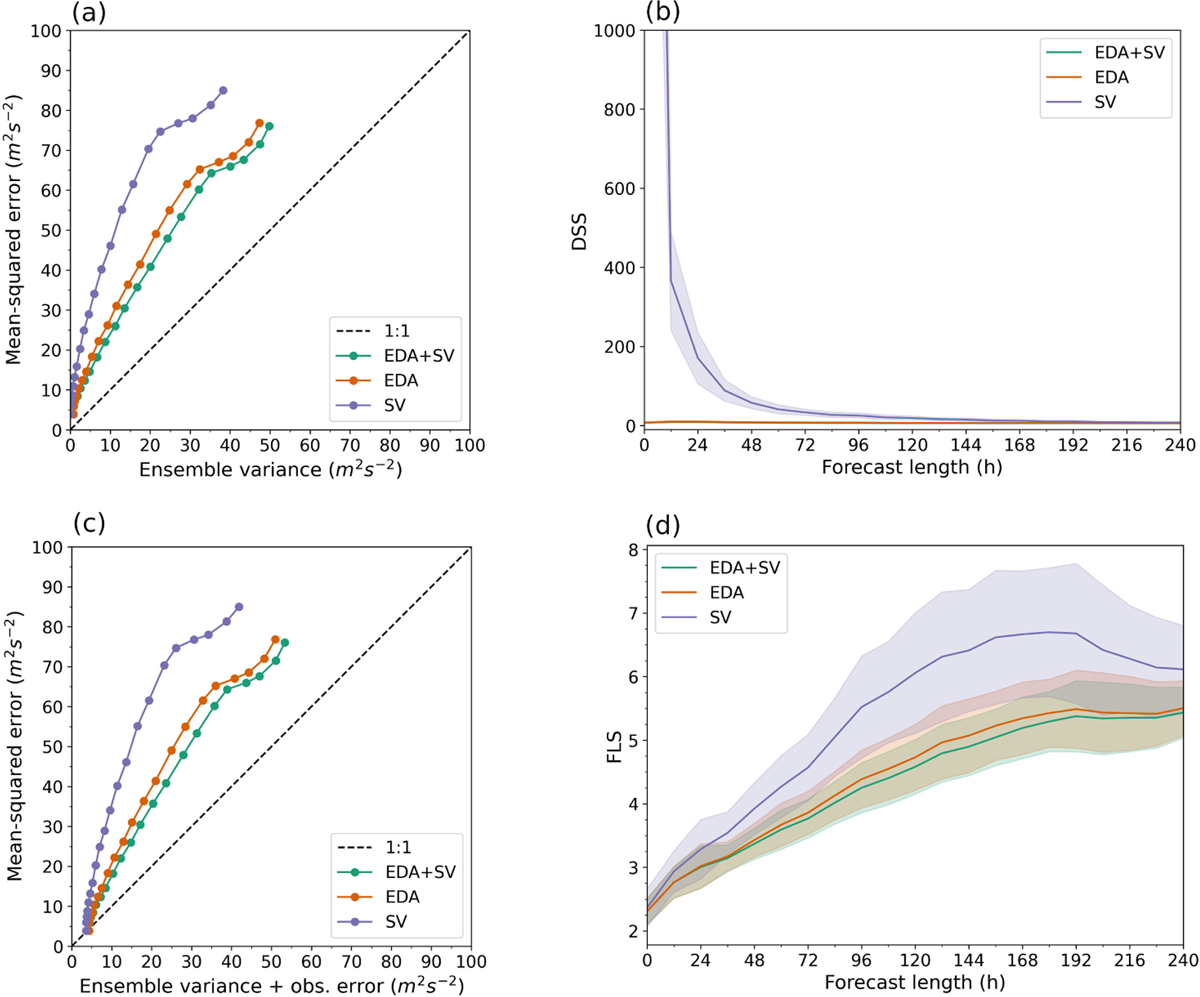
Figure 5
Different verification metrics for u500 in NH. Comparison between different verification metrics for wind component u at 500 hPa in the Northern Hemisphere: (a) Ensemble spread-skill relationship, (b) Dawid-Sebastiani score, (c) Ensemble spread-skill relationship with observation error, and (d) Filter likelihood score. The solid lines show the mean value of the metric and the shaded area one standard deviation uncertainty. The green line shows forecasts with EDA and SV initial conditions, orange with EDA, and purple with SV. The dots in panels (a) and (c) show the spread (+obs.error)/error relationship for different forecast lead times every 12h.
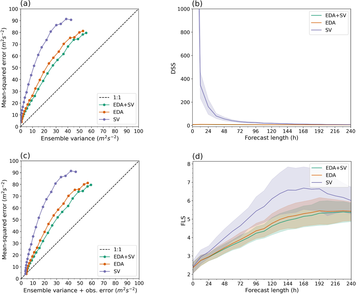
Figure 6
Different verification metrics for v500 in NH. Comparison between different verification metrics for wind component v at 500 hPa in the Northern Hemisphere: (a) Ensemble spread-skill relationship, (b) Dawid-Sebastiani score, (c) Ensemble spread-skill relationship with observation error, and (d) Filter likelihood score. The solid lines show the mean value of the metric and the shaded area one standard deviation uncertainty. The green line shows forecasts with EDA and SV initial conditions, orange with EDA, and purple with SV. The dots in panels (a) and (c) show the spread (+obs.error)/error relationship for different forecast lead times every 12h.
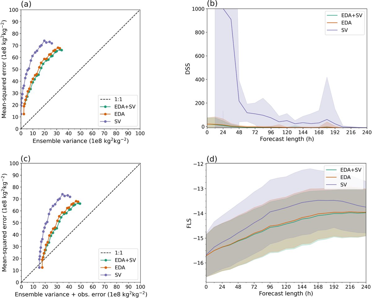
Figure 7
Different verification metrics for q500 in NH. Comparison between different verification metrics for specific humidity q at 500 hPa in the Northern Hemisphere: (a) Ensemble spread-skill relationship, (b) Dawid-Sebastiani score, (c) Ensemble spread-skill relationship with observation error, and (d) Filter likelihood score. The solid lines show the mean value of the metric and the shaded area one standard deviation uncertainty. The green line shows forecasts with EDA and SV initial conditions, orange with EDA, and purple with SV. Please note that in panel (a) and (c), the values are multiplied by 108. The dots in panels (a) and (c) show the spread (+obs.error)/error relationship for different forecast lead times every 12h.
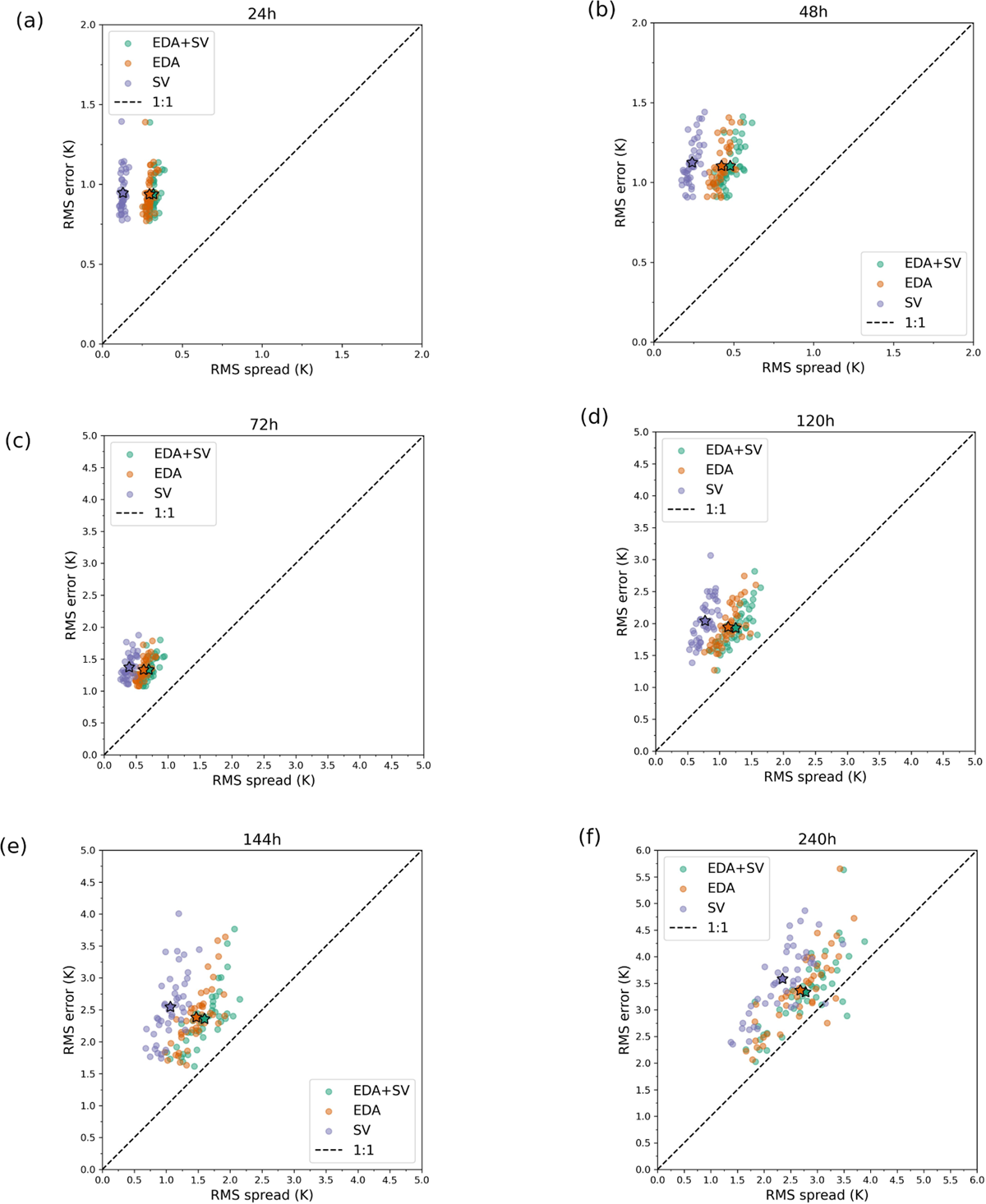
Figure 8
Root-mean squared (RMS) error versus spread for temperature at 500 hPa at different forecast lead times (a) 24h, (b) 48h, (c) 72h, (d) 120h, (e) 144h, and (f) 240h. One dot represents the RMS error/spread relationship for one ensemble forecast and the star is the mean over all ensembles. Green shows EDA+SV ensembles, orange EDA ensembles, and purple SV ensembles. The mean RMS error/spread relationship (marked with stars) corresponds to the dots in panel (a) of Figure 1.
If we assume Gaussian error models for both model error and observations, the filter based likelihood in (A3) will be just like in equation (3)
Here, the approximation comes from the fact that we are using a finite ensemble to calculate empirical mean and covariance and linearised versions of the non-linear operators and .
The original reference for filter likelihood comes from Schweppe (1965) and a more detailed derivation than the one given above is given in (Särkkä 2013). In this article the likelihood is used as a verification score by normalising it with the number of observations. We are interested in the relative score of the forecast system given the observations, when comparing different systems or perhaps monitoring the performance over time. In the case contains tunable parameters θ, the likelihood provides means of objective model tuning. This was done, for example, by Hakkarainen et al. (2012) to tune closure parameters in forecast models. Solonen and Järvinen (2013) used likelihood score to tune parameters related to the ensemble system and Ekblom et al. (2020) used Kalman filter likelihood cost function to tune the spread–skill relationship of an ensemble forecasting system.
Acknowledgements
The authors wish to acknowledge CSC – IT Center for Science, Finland, for computational resources. The authors want to thank Reima Eresmaa for help with downloading the observations from MARS, Heikki Haario for useful discussions while preparing and writing this paper, and Peter Bechtold and Niels Bormann for the idea of using the Radiance Simulator software for the computation of the model counterparts for AMSU-A channel 5 observations. We would like to thank the two anonymous reviewers for their constructive and useful comments that helped to improve the manuscript.
Funding information
We would like to acknowledge the funding from the Academy of Finland (grant nos. 333034, 316939, 321890 and 348092) and the doctoral programme in atmospheric sciences at the University of Helsinki, Finland (ME and LT). We would like to acknowledge funding received from the European Union’s Horizon 2020 research and innovation programme under grant agreement No 101003826 CRiceS (PO) and No 101003470, the NextGEMs project (ME, LT, and HJ) as well as from the Vilho, Yrjö and Kalle Väisälä Foundation of the Finnish Academy of Science and Letters (ME).
Competing Interests
The authors have no competing interests to declare.
Author Contributors
ME implemented the verification metrics with help from OR and ML and performed the analysis of the verification metrics. LT calculated the model counterparts for the satellite observations. PO assisted with the forecast data. ML and HJ supervised the work. All authors contributed to the discussions on the results and to the writing of the manuscript.