
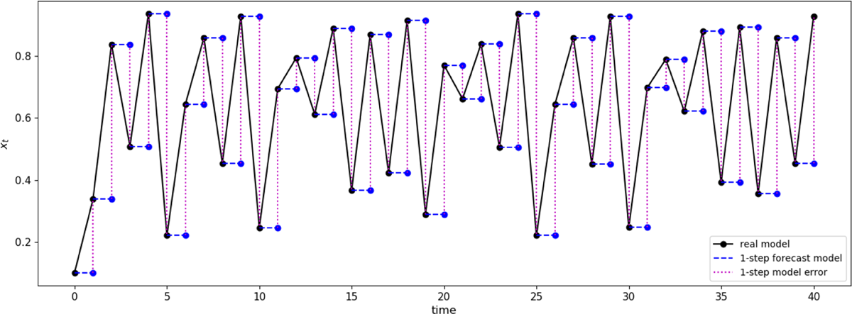
Figure 1
Simple illustration for the origin of auto-correlated model error. The system evolves under a real system represented by the logistic map (black line). 1-lag forecasts are produced with an imperfect model (blue line), persistence. The 1-lag model errors are computed by taking the differences of the two values (dashed magenta lines).
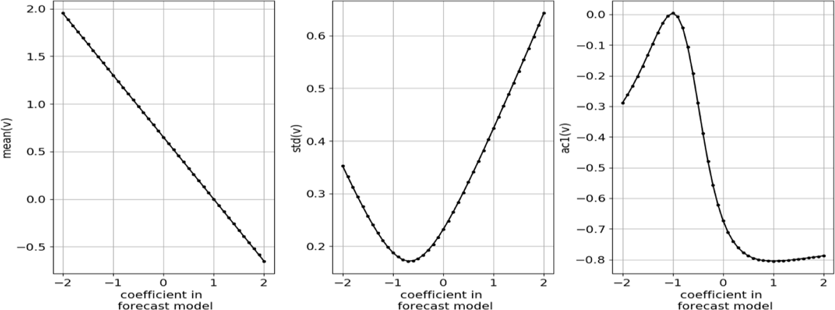
Figure 2
Model error statistics (mean in left panel, standard deviation in centre panel, lag-1 auto-correlation in the right panel). These statistics are computed off-line, after a long model run, in the way illustrated in figure 1. These are computed for different coefficients in the forecast model (horizontal axis in panels).
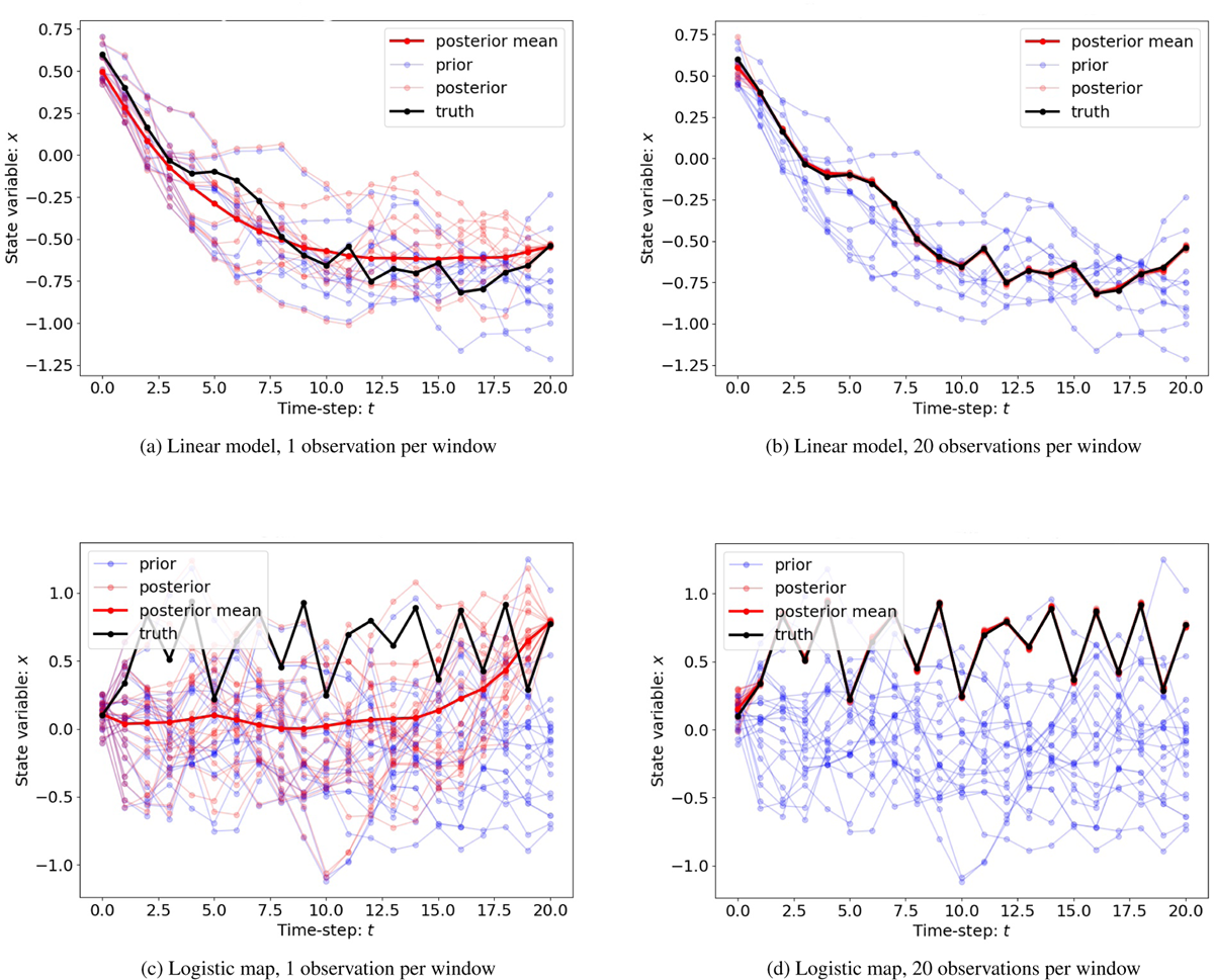
Figure 3
State update for both linear model and logistic map with different number of observations over a single simulation window using EnKS.
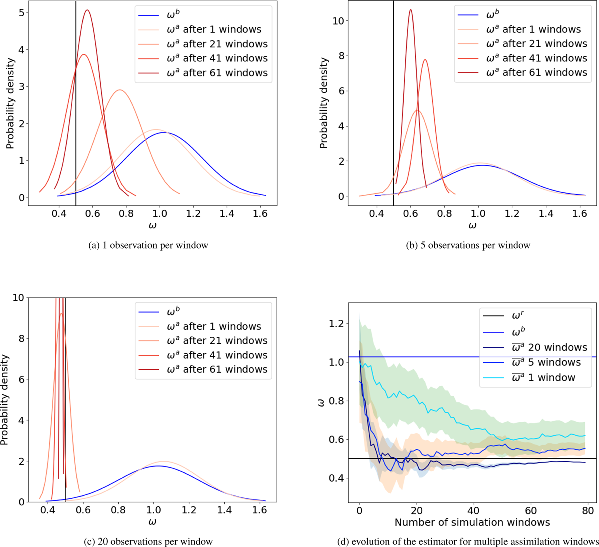
Figure 4
(a)∼(c) Exponential scale estimation with different numbers of observations and simulation windows using the EnKS and (d) the convergence of the mean of posterior pdf with the number of simulation windows.
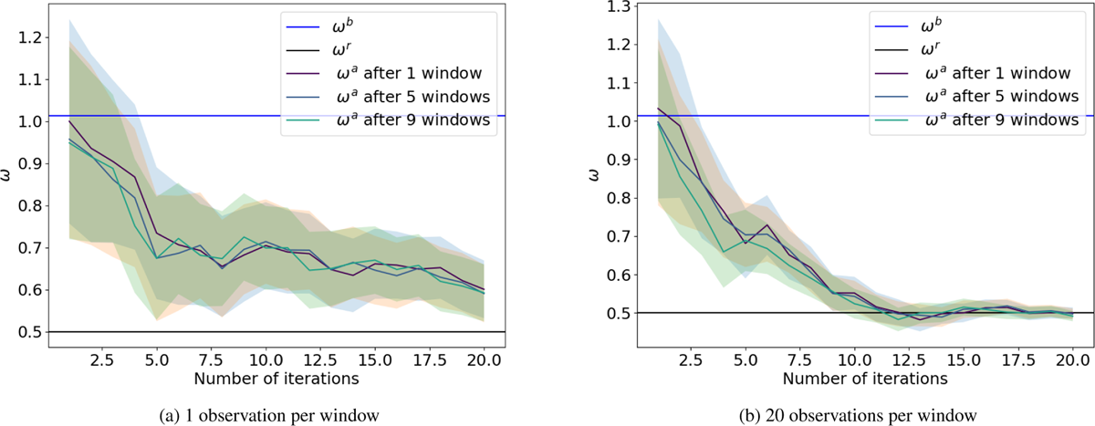
Figure 5
Analysis mean and standard deviation resulting from using IEnKS with different number of observations (panels), iterations (horizontal axis), after different number of simulation windows (lines).
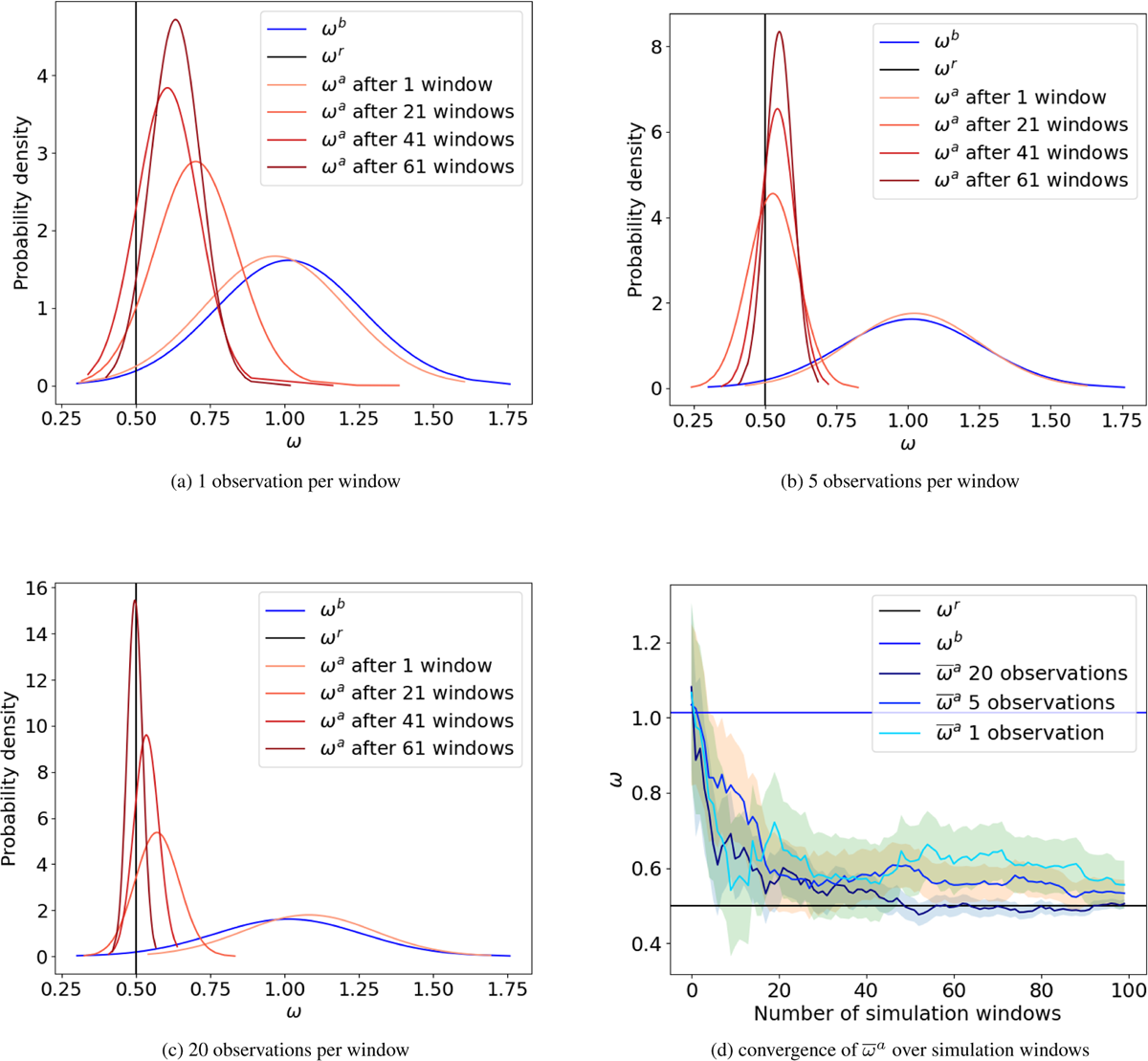
Figure 6
(a)∼(c) Exponential scale estimation with different numbers of observations observations and simulation windows using IEnKS and (d) the convergence of the mean of posterior pdf with the number of simulation windows.
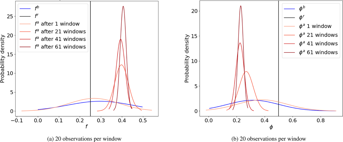
Figure 7
Two-parameter estimation, f (left) and φ (right), using the EnKS with 20 observations and different number of simulation windows.
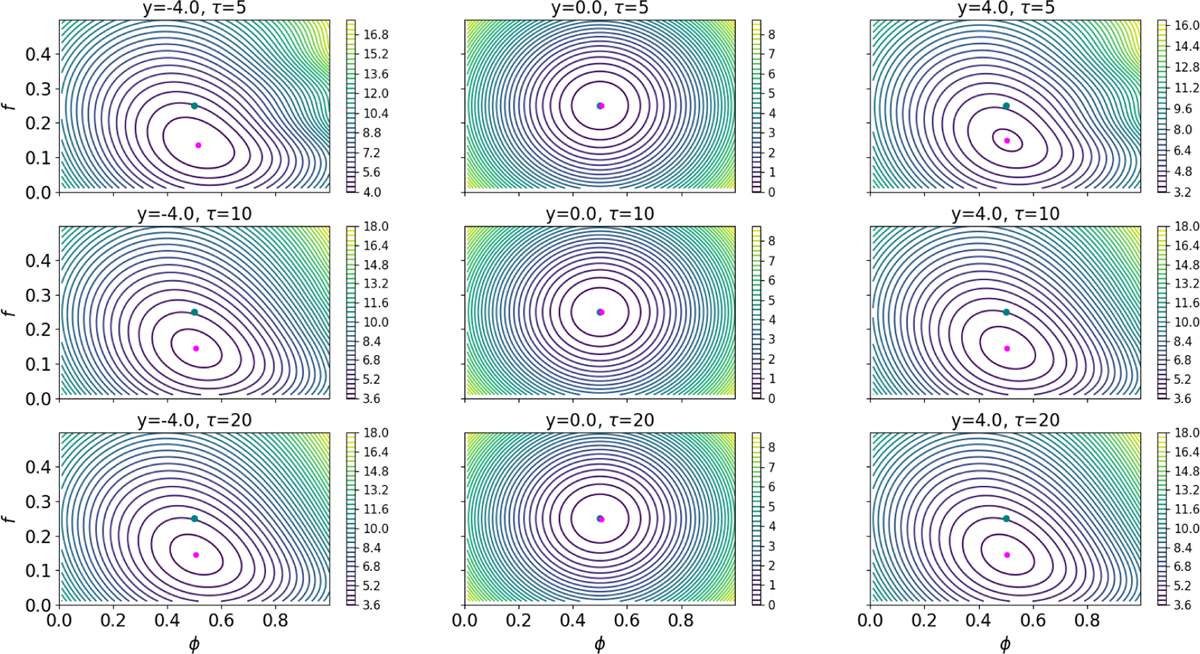
Figure 8
Exact cost function including the two-parameter model error, the state variable, observations with different number of time-steps and values of observations using the EnKS. The blue point represents the analysis value predicted after 1 EnKS step (with no extra iterations), and the pink point represents the exact global minimum.
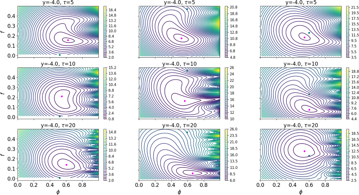
Figure 9
Sample cost function of different ensemble members (from left to right, Ne = 2,4,8) including the two-parameter model error, the state variable, observations with different number of time-steps and values of observations using the EnKS. The blue point represents the analysis value predicted after 1 ENKS step (with no iterations), and the pink point represents the exact global minimum.
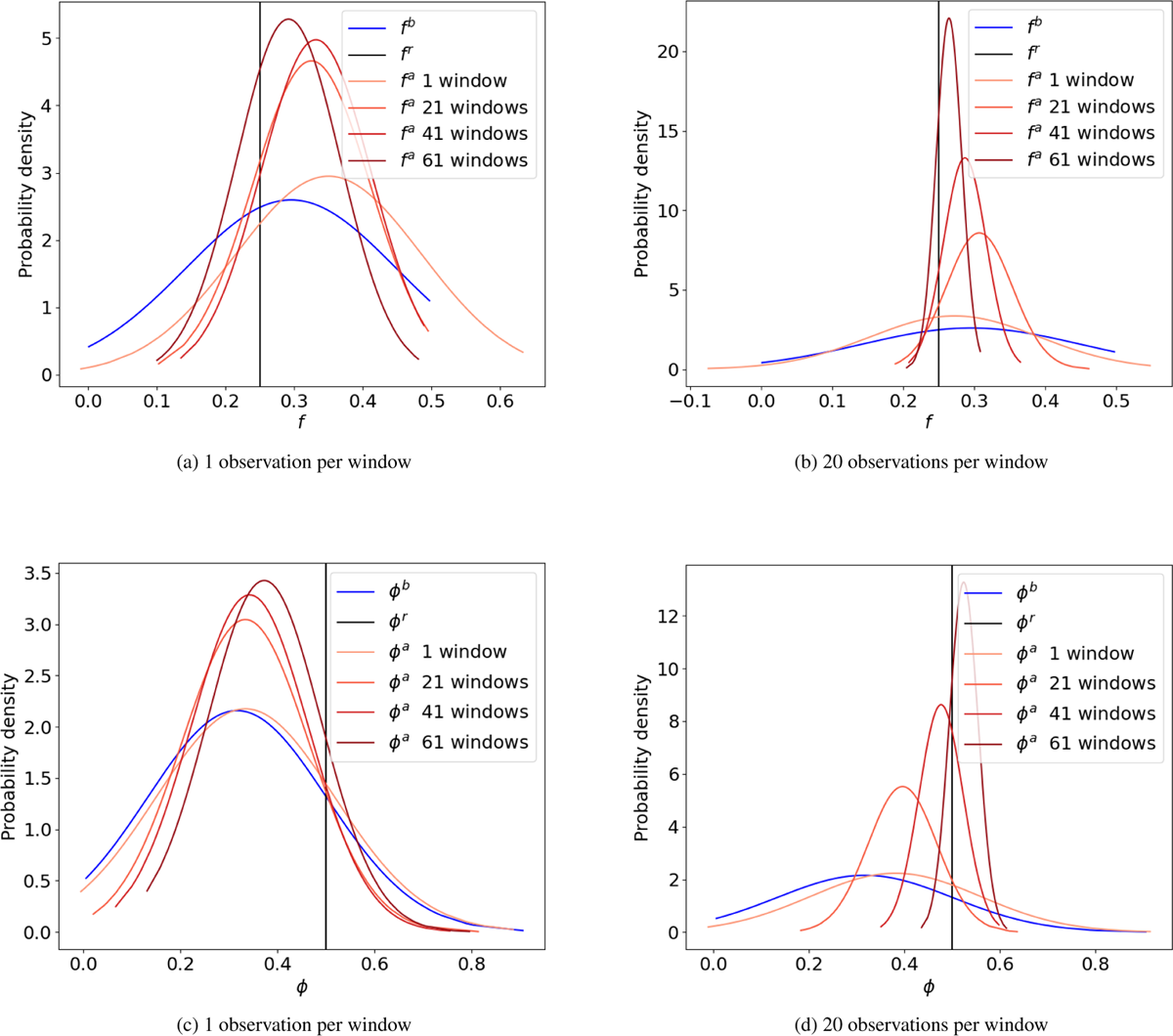
Figure 10
Two-parameter estimation using the IEnKS with different number of observations and simulation windows, and 10 iterations.
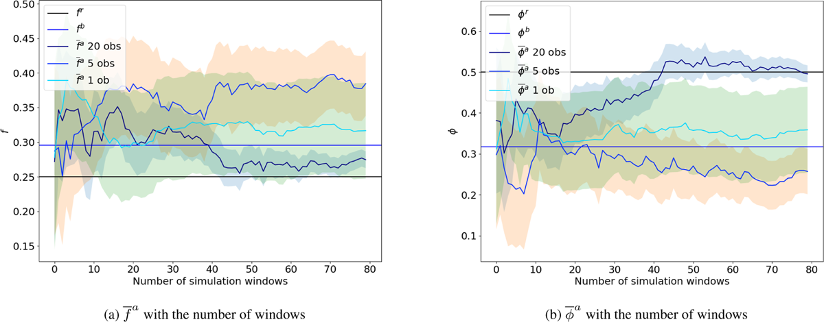
Figure 11
Posterior mean of the two parameters over the number of simulation windows with different number of observations.
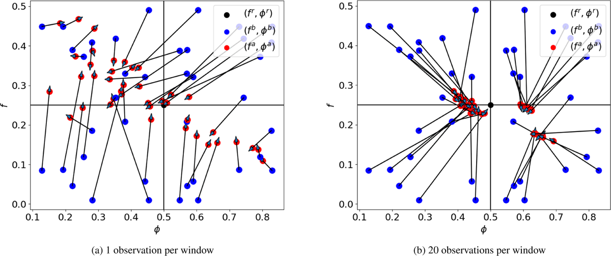
Figure 12
Two-parameter estimation for different priors using the IEnKS with different number of observations and simulation windows after 10 iterations. The blue dots show different background values, used as initial conditions for the minimisation. The red dots show the obtained analysis values. The black dot in the centre shows the true values for the parameters.
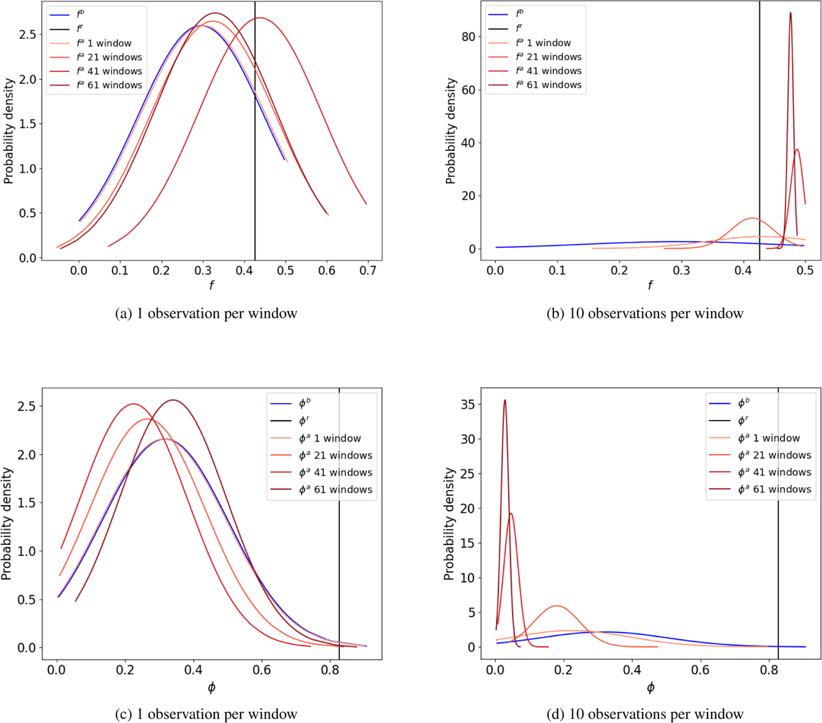
Figure 13
Two-parameter estimation using the IEnKS with the logistic map, using a fixed iteration step length (δ = 0.3), 10 iterations per window, different number of observations and simulation windows.
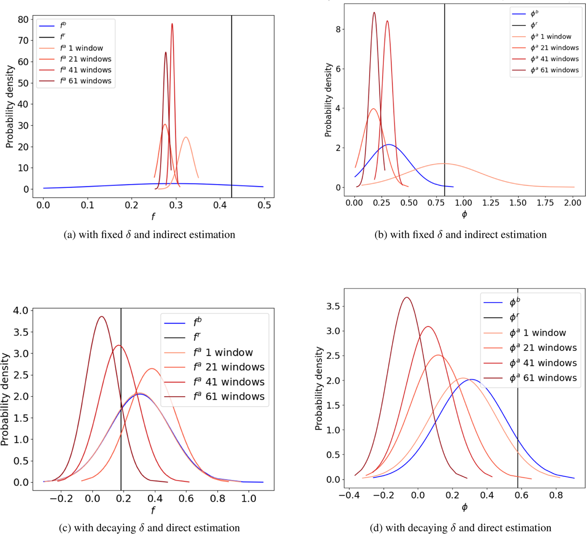
Figure 14
Two-parameter estimation using the IEnKS with 10 observations per window after 10 iterations with the logistic map. On the top panel, (a)∼(b) the iteration step-length is fixed (δ = 0.3), and we estimate the lag-1 and lag-2 autocorrelation then transform them to f and φ. On the bottom panel, (c)∼(d) the parameters are estimated directly with a decaying δ.
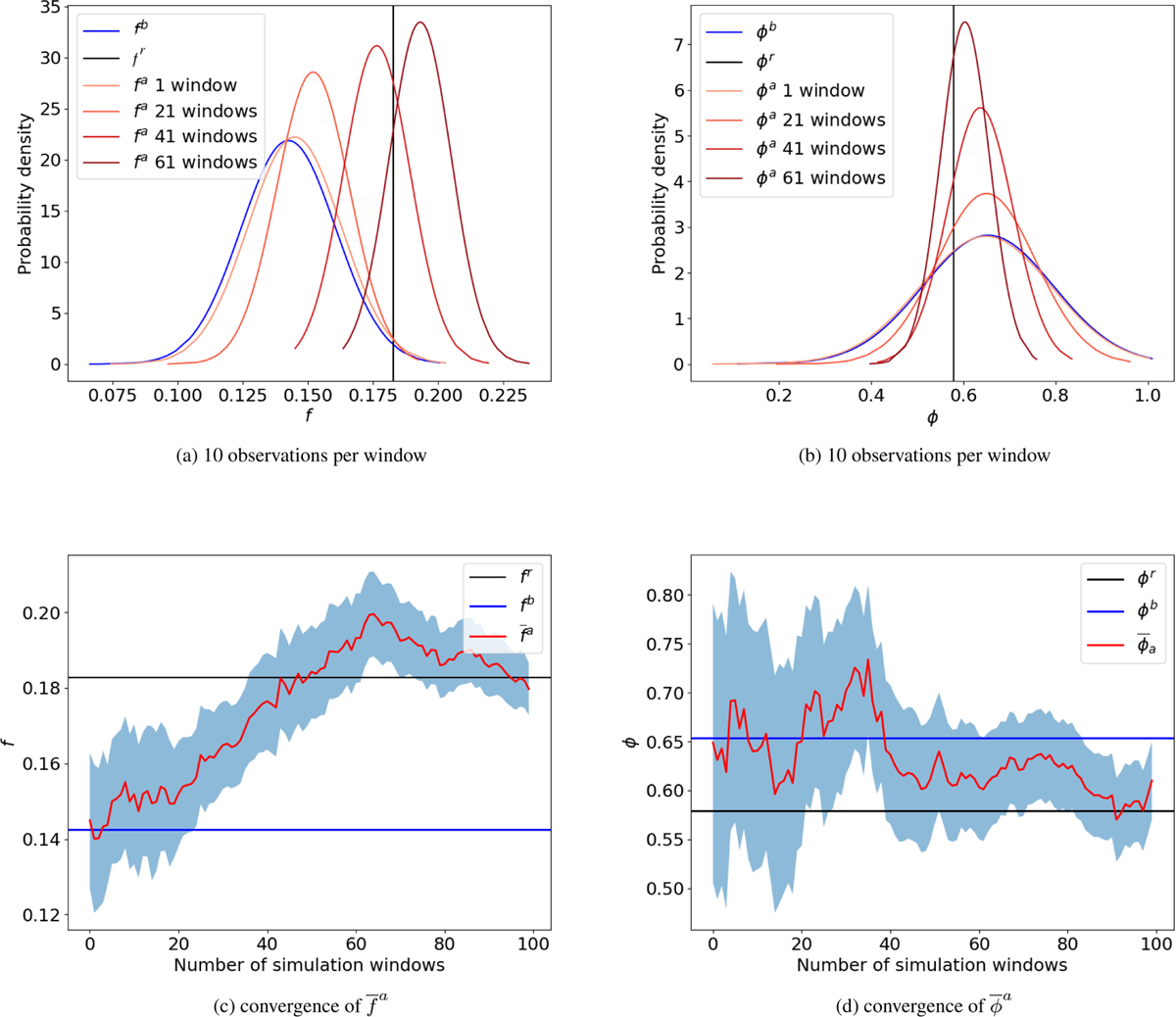
Figure 15
Lag-1 and lag-2 autocorrelation are estimated and transform to the parameters (a) f and (b) φ, using the IEnKS with a decaying iteration step length, 10 iterations per window, for different numbers of assimilation windows with the logistic map. The bottom two figures show the convergence of the posterior mean of (c) f and (d) φ over the number of simulation windows with observations every time-step.