
1 Introduction
Data assimilation (DA) combines observations –obtained from the real world– with a numerical forecast to improve the accuracy in the estimation of the state of a system. This new estimate acts as initial condition for new forecasts, see e.g (Asch, Bocquet, and Nodet, 2016; Evensen, Vossepoel, and Leeuwen, 2022) for a complete overview. Forecast models have often been considered perfect representations of the processes in the real world, the so-called strong constraint in the DA literature. This leaves the uncertainty in initial conditions as the sole culprit for any forecast errors. In reality, however, model error can become as important as initialisation error in degrading forecast accuracy (Orrell et al., 2001). In numerical weather prediction (NWP) systems, model error arises from time and space discretisations, approximate parameterisations of physical processes that are not represented explicitly, unresolved sub-grid processes, etc. While these errors are often ignored in the DA process, it is common knowledge that more accurate solutions can be obtained if they are included.
Due to limited computational power and insufficient observations from reality, model error was originally considered in relatively simple cases, extending from one-dimensional systems to two-dimensional shallow-water systems (see e.g seminal papers by Ghil et al., 1981; Cohn and Parrish, 1991). Later, the increase in computational power and in knowledge of the model error allowed for the successful application of weak constraint DA into more complex models (Ghil, 1989; Tremolet, 2006; Palmer et al., 2009; Berner et al., 2017; Howes, Fowler, and Lawless, 2017; Evensen, 2019). For simplicity, model error has often been treated as a random variable with Gaussian distribution and no time auto-correlation in time, i.e. white in time. The reality can be quite different. The impact of model error caused by unresolved processes on the forecast and DA results can last for several model time steps. Bennett (1992), typically way ahead of his time, extensively discussed the use of correlated model errors and solution of the problem using the representer method, Amezcua and Van Leeuwen (2018) formulated the time-correlated problem for ensemble smoothers, and Evensen (2021) extended this to iterative ensemble smoothers. An obstacle in this endeavor, however, is that it is hard to describe a prior on the model errors, especially if one is to include non-trivial probabilistic elements in both space and time. As a result, there has been interest in estimating model errors in DA schemes in the last two decades (Brasseur et al., 2005; Crommelin and Vanden-Eijnden, 2008; Zhu, Van Leeuwen, and Zhang, 2018; Lucini, Leeuwen, and Pulido, 2019; Bonavita and Laloyaux, 2020; Brajard et al., 2021; Pathiraja and Leeuwen, 2022; Evensen, 2021).
Let us provide a simple illustration of the way time auto-correlated model error arises. Consider the time evolution of the logistic map with coefficient γtrue = 3.75, which is shown in Figure 1. This zero-dimensional non-linear discrete map was made popular by Robert (1976), and is described with more detail in section 3. The nature (or true) evolution is shown by the black solid lines and the black dots. Now, consider an imperfect forecast model. The simplest one we can think of is persistence, i.e. no evolution over one model time step. If we take the exact values of the nature run at every model time step, and evolve them with this imperfect forecast model over one step, we obtain the blue lines. Taking the difference between the true value of the variable and the imperfect 1-step forecast renders the dashed magenta lines. These are 1-step model error values diagnosed offline, and therefore useful only retrospectively.
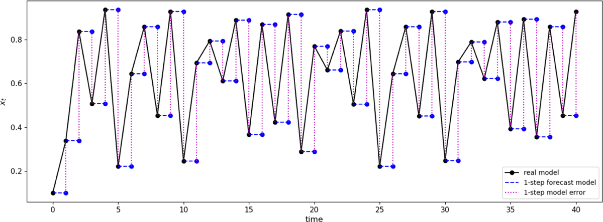
Figure 1
Simple illustration for the origin of auto-correlated model error. The system evolves under a real system represented by the logistic map (black line). 1-lag forecasts are produced with an imperfect model (blue line), persistence. The 1-lag model errors are computed by taking the differences of the two values (dashed magenta lines).
To characterise this model error, we run the described process for a long time period (104 model steps), save the model error values for each time step, and compute statistics on these values (similar to Evensen and Fario, 1997). Figure 2 shows three statistics: mean (left panel), standard deviation (centre panel), and lag-1 auto-correlation (right panel). To make the experiment more general, we keep the true model fixed, but in the forecast model we vary the coefficient multiplying the value in the previous time step (persistence is when the coefficient is one). In each panel, the horizontal axis corresponds to values of this coefficient, while the vertical axis corresponds to the value of the statistic. The three statistics vary as function of the coefficient in the forecast model. Moreover, the lag-1 auto-correlation shows a non-trivial behaviour, and is zero in only one occasion. Hence, only for a very particular coefficient choice the model error is independent in time, and in general it is not. This model error has been diagnosed offline. The question we aim to answer is whether it is possible to obtain these estimates online.
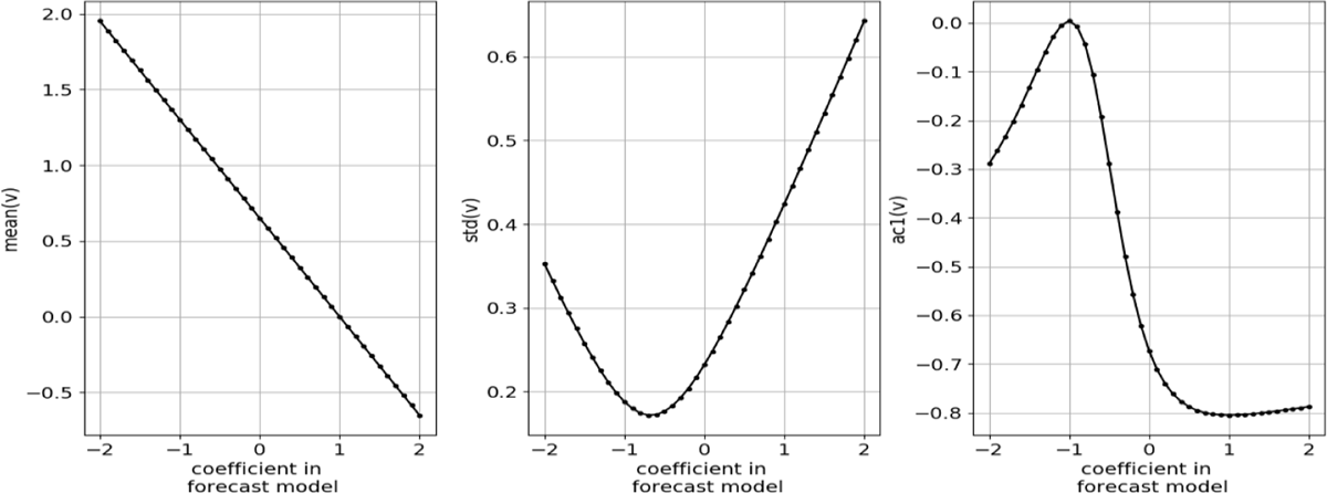
Figure 2
Model error statistics (mean in left panel, standard deviation in centre panel, lag-1 auto-correlation in the right panel). These statistics are computed off-line, after a long model run, in the way illustrated in figure 1. These are computed for different coefficients in the forecast model (horizontal axis in panels).
A previous work (Ren, Amezcua, and Van Leeuwen, 2021) investigated the impact of time auto-correlated model error in DA. The current work has the specific objective to perform online estimation of the time-related characteristics of this model error. Our goal is to improve the accuracy of the forecast by sequentially updating the error using an ensemble Kalman-based method (Kalman, 1960; Kalman and Bucy, 1961). In particular, we use the Ensemble Kalman Smoother (Evensen and Van Leeuwen, 2000; Evensen, 2018; Amezcua and Van Leeuwen, 2018). As a smoother, instead of only updating fields at observation time, it updates the whole trajectory over a simulation window using all available observations in that window. The EnKS uses ensemble integrations to approximately represent the density for the prior model evolution. This ensemble is then used to solve the DA problem under the Gaussian assumption for model states, parameters and observation errors, and an observation operator that does not deviate too much from linear. Ren, Amezcua, and Van Leeuwen (2021) performed parameter estimation for the model error with spatial and temporal autocorrelation using an EnKS, and, while successful in some cases, the parameter estimation failed in others. It was argued that the failures were due to the linear correlations that are assumed in an EnKS. We will investigate this claim by using a nonlinear iterative EnKS (IEnKS) (Sakov, Oliver, and Bertino, 2012; Evensen, 2018). The IEnKS can be regarded as an ensemble variational method that does not require the tangent linear of the evolution and observation models, nor the adjoint of these models (Bocquet and Sakov, 2014).
This paper is organised as follows. In section 2 we show how the problem of jointly estimating state variables and time-related parameters in the model error is a difficult one. We show that even when the state variables follow linear dynamics, the time-related model error parameters appear in a very non-linear fashion within the associated cost function. This complicates the estimation problem, and makes that the minimum variance and maximum a posteriori solutions differ considerably. In practice, it requires the use a nonlinear DA method such as the IEnKS for the joint estimation problem. In section 3 we describe our experimental setup. We choose two types of memory for the model error: one with pure exponential decay, and one with a mixed oscillatory-exponential decay. In this section we also describe the two models used in our experiments: the simple model of section 2, and also the logistic map, which provides insight into what happens with non-linear dynamics. Results of these experiments are presented and discussed in section 4. Finally, section 5 provides a summary and discussion of the work.
2 Estimating auto-correlated model error in a simple linear model
Estimating model error is a difficult problem, especially when these errors are correlated in time. We explore a systematic approach in which we aim to estimate parameters of the time-correlation part of the model error formulation. Specifically, we assume a model error structure that is separable in space and time. We parameterise the time-dependent behaviour with decaying and oscillatory parameters, and then use use DA to estimate them.
This section illustrates how the parameters related to time-dependent model error are involved in a nonlinear manner in the imperfect model evolution. Therefore, the online estimation of these parameters becomes a challenge for Bayesian estimation. For simplicity, let us consider zero-dimensional systems, which serves two purposes. First, it allows for analytic steps to be feasible and provide important insight. Second, we do not need to worry about spatial structures in the model error and can focus on the time structures.
In the following we first formulate the problem of jointly estimating state variables and parameters, followed by the full Bayesian problem set up. We show that, because the time-related parameters in the model error are related nonlinearly to the state variables, the parameter estimation problem is always nonlinear, even when the prior on the paramaters is Gaussian and the model is linear in the state. Then we formulate two solutions, one that finds the mode of the posterior, and the other first linearizes the problem and then finds the mean. The solution without linearization will be more accurate, but also much more computationally expensive as it relies on an iterative procedure that employs the adjoint model, and does not easily provide an error estimate. The solution to the linearized problem is computationally much more efficient, but differs significantly from the solution to the nonlinear problem. We then formulate an iterative ensemble method, which is a more accurate solution to the full nonlinear problem. No explicit solution exists for this ensemble method, but the method is computationally efficient. This is the method we use in our numerical experiments we perform to achieve online estimation.
2.1 Problem formulation
Let be the state variable of our system with initial conditions x0 at t = 0. Consider τ independent model error jumps ϵt, for t = {1,…,τ} with zero mean. We denote the control variable as the column vector , with background distribution :
where and are the background mean vector and background error covariance matrix, respectively. The scalars b2 and q2 represent the background and model error variances. Note that z has a diagonal covariance matrix since we consider statistical independence amongst its elements. We use these elements to construct a simple linear system with time auto-correlated model errors in its evolution. The real linear evolution over one time step is prescribed by:
i.e. a simple auto-regressive component plus a model error realisation. This model error has distribution v(t) ~ N (0,q2), and the following structure in time:
Eq. (3) indicates that the model errors are auto-correlated in time, and this only depends on the lag |t–t|′ and a vector of Nθ parameters . For τ time steps, this yields an auto-correlation matrix . This symmetric Toeplitz has the following elements:
Being a positive-definite symmetric matrix, a Cholesky decomposition Φ is possible, i.e.:
where is lower triangular.
We now take Eq. (2) and write the time evolution of the system from t = 0 to t = τ in terms of the control vector z and the Cholesky factor L. Explicitly:
where is a row matrix with the model evolution from 0 to any time t. For this simple model, the elements are decreasing powers of α:
Let us define the composed evolution matrix :
This includes the effect of the deterministic dynamics and the auto-correlation of the model error, and it will become useful in the next subsections. Separating the initial condition and the model errors, we write Eq. (6) as:
where and are obtained by removing the first element of M0:τ and z respectively. In fact, we can recover the value xt at any time (not just the final time) using with the corresponding truncated elements in the second term.
We consider an observation of the truth at the end of the forecast window, i.e. at time t = τ. For simplicity, let the observation operator be the identity, so the observation equation is:
with the observation error: η ~ N(0,r2). Obtaining the analysis values for z was already discussed in Amezcua and van Leeuwen (2018), and Ren et al (2021). In this paper we discuss the solution of the joint state-variable estimation problem.
2.2 Bayesian solution for the joint state-parameter estimation
Considering both the control variable z and parameters θ to be random variables, the Bayesian solution of this problem is to obtain the posterior joint pdf of z and θ given the observation y. Namely,
The numerator is the joint pdf of z, θ and y. This is obtained as the product of the likelihood of y times the prior joint pdf of z and θ. If we consider these two to be statistically independent, then we have:
The marginal pdf of the observations is:
The prior distribution for the control variable and the likelihood are easy to characterise. Recall that we have:
From now on, we explicitly note that depends on θ. Note that the joint estimation problem is complicated since we have the product in the likelihood, which limits the possibility of obtaining an analytical expression for the posterior p(x,θ|y). For this reason, we now discuss two solutions based in statistics of this pdf: the maximum-a-posteriori solution, and a popular approximation, the extended Kalman smoother solution.
2.3 The Maximum-a-posteriori solution
We can try maximising the joint pdf to obtain a maximum-a-posteriori (MAP) solution. This is equivalent of finding the minimum of the cost function:
Using the distributions in Eq. (14) and an arbitrary prior for θ, the minus logarithm of Eq. (12) is:
The minimisers {z*, θ*} of the cost-function can be obtained by taking the gradient of J(z, θ|y) with respect to both control variables and parameters and equating to zero:
with the gradients and . If we also assume that the parameters follow a MVG –i.e. θ ~ (µθ, Dθ)– we are able to compute the gradients explicitly. This yields the following system of τ + 1 + Nθ equations:
with the Jacobian matrix defined as:
One can solve z from Eq. (18a) to get:
with K and γ2 defined as
and similarly from Eq. (18b):
Eq. (20) is the Kalman analysis equation for the posterior mean (Kalman, 1960; Kalman and Bucy, 1961). The complication, however, is in our case θ is an unknown. Hence, Eq. (20) needs to be solved in tandem with Eq. (22), which cannot be done analytically in general.
To actually calculate the derivative of the model with respect to the parameters, we note the following. For the jth parameter θj, Eq. (19) can be readily computed using the Cholesky factor L defined in Eq. (5) in the following manner:
The derivative of the Cholesky matrix can be found using Theorem A.1 of Sarkka (2013):
where the matrix is defined as:
2.4 The extended Kalman Smoother solution
The extended Kalman Smoother solution can be derived directly from the MAP solution by centering the derivative of the model to the state and the parameters on the background values. Tracing back these derivatives we can rewrite Eq. (20) and Eq. (22) as:
Furthermore, in Eq. (27) we use a first-order Taylor expansion for as:
We can solve then solve Eq. (26) and Eq. (27) by introducing a new augmented variable and after some algebra we obtain:
where Az is denoted as the posterior covariance in the extended variable space. In this case, the augmented gain and augmented residual variance are different from Eq. (21)
In the last step we have again assumed that state variables and parameters are statistically independent in the prior. Notice that even with a Gaussian prior p(θ) and a model that is linear in the state z the MAP and the extended KS solution can differ considerably. The MAP solution results in an implicit equation that needs to be solved iteratively. However, even if we manage to do this an uncertainty estimate is still lacking. It is possible, if the system is low-dimensional, to solve this problem with e.g. a particle filter. Unfortunately, for higher dimensions particle filters are degenerate, and a potential solution for that, localization, is difficult to use with global parameters. Instead, we resort to a popular approximate solution based on an iterative Ensemble Kalman smoother that can easily be scaled up to higher dimensions.
2.5 The (Iterative) Ensemble Kalman Smoother
The Iterative Ensemble Kalman Smoother (IEnKS) does solve the parameter estimation problem approximately, but it does introduce nonlinearity in the solution procedure. Hence it will provide a solution that is closer to the MAP solution than the Extended Kalman Smoother solution. In an IEnKS parameter estimation is typically performed via state augmentation, as in the extended Kalman Smoother. We define a variable as:
where the augmented variable includes the state variable at all time steps and all the model error parameters, sometimes called the state formulation. Notice that this is slightly different than Eq. (1), where the augmented variable contains the initial conditions, the model error jumps, and the model error parameters, leading to the so-called forcing formulation. In a linear system, it is trivial to go from one formulation to the other, as explained in Tremolet (2006) and Amezcua and Van Leeuwen (2018). For ensemble implementations it is easier to work with state variables directly, so this is how we implement the experiments in the paper.
Ren, Amezcua, and Van Leeuwen (2021) studied the consequences of wrongly prescribing the model error decorrelation time scale, which was the only parameter. This is, they performed DA with a model error auto-correlation which was different from the one ‘guessed’ in the ensemble forecast. In the last part of the work, they used state augmentation in an EnKS –as formulated in Amezcua and Van Leeuwen (2018)– to estimate one time parameter in the model error. The authors did not, however, perform a systematic analysis with different types of model error structure. In this work we perform a deeper analysis and more extensive experiments.
In this work we perform state augmentation experiments using two DA methods, the stochastic EnKS and its iterative variant (IEnKS), as formulated in Evensen (2018). This formulation aims to find the minimum of a cost function using ensemble members, either in one step (EnKS) or multiple steps (IEnKS). In the IEnKS a cost function is defined for each ensemble member j by rewriting the cost function Eq. (16) in terms of the extended variable u as:
in which is the prior ensemble member j, and
is a perturbed observation with the perturbation drawn from the observation error pdf, so ηj ~ N(0,r2). In Eq. (32) it is clear that the product is responsible for the difficulty of this problem. Evensen (2018) proposed a simple Gauss-Newton iteration for each ensemble member as:
where i is the iteration index, is a symmetric approximation of the Hessian of the cost function in which the second derivative of is neglected, so
and is the gradient of the cost function for ensemble member j. The iteration step length δ is tunable. The iteration is started at . The simple descent algorithm can be used with the ensemble gradient and the ensemble approximated Hessian information, as shown in equation (36) of Evensen (2018). For efficiency, we use the particular implementation described in Evensen et al. (2019). Tuning factor δ is an art. In our implementation we reduce the step size the closer we get to the minimum via:
with 0<c<1. The stochastic EnKS can be obtained from this formulation by using only one iteration and setting δ = 1.
3 Experimental setup
For our experiments, we use two types of model error (with one and two parameters), and two types of evolution models (linear and nonlinear).
3.1 Model error formulations
The first type of model error was used both in Amezcua and Van Leeuwen (2018) and Ren, Amezcua, and Van Leeuwen (2021). The correlation of model error between two time steps is:
In this case, the auto-correlation decays exponentially, and it only has one parameter – the decay time scale ω (ω>0). When ω tends to 0 the model error becomes a white-noise process. When ω tends to infinity, the model error becomes fixed (a bias). Summarizing:
The second model error structure we explore contains both decaying and oscillatory elements:
The first term is a geometric memory term, with base –1 < φ < 1, which can be considered a decay parameter. The second term is oscillatory with frequency f. To avoid instability of the system, the decay parameter φ is bounded as 0 ≤ φ ≤ 1, and the frequency f is bounded by 0 < f < 0.5. When the frequency is 0.5, the covariance becomes purely decaying with time and it becomes purely oscillatory when the decaying parameter tends to 1.0. Summarising:
3.2 Evolution models
To illustrate the issues that arise when estimating model error parameters that are related to temporal correlations, we restrict our experimental set up to two zero dimensional models. The first is the simple linear scalar model used for the analysis in section 2. The true model is:
Note that this true model is a stochastic model and we assume v ∼ N(0,q2). The true model uses a real decay timescale ωr, while the forecast model assumes a guessed time auto-correlation parameter ωg. This value needs to be updated in the DA cycle.
The second set of experiments is much more ambitious since we use a non-linear map as the real system. In particular, we use the well-known logistic map (Robert, 1976):
where γ is the control coefficient that gives rise to stable solutions when 0 ≤ γ ≤ 4; by stable we mean solutions that do not leave the interval [0,1]. In our experiments we choose γ = 4 which puts the model in a chaotic regime. Note that in these experiments, the true model is deterministic. This seemingly simple non-linear map is non-invertible, with initialisation errors growing and saturating quickly. It has therefore been used before to test the performance of different configurations of the EnKF (Mitchell and Houtekamer, 2009). The true autocorrelation of the model error (computed offline as described in the introduction) has both positive and negative values, while decreasing in absolute magnitude as a function of the lag. Therefore, a 2-parameter memory is more appropriate for this case, although it increases the difficulty of the problem by having to estimate an extra parameter.
As a forecast model, we propose a stochastic linear model
where γg is a prescribed damping coefficient for the forecast model, with its value within 0 < γg < 1 to keep the model stable. The model error has the same properties as in the experiments where the real model is linear. In section 1, we described an off-line process to compute the statistics of this model error from a long-time collection of differences between perfect and imperfect forecasts. What we look for, instead, is to estimate the time-related parameters online, along with the state estimation.
3.3 Implementation details
Our experiments follow the fraternal (non-identical) twin set up. A real initial condition is prescribed and the true model is run for a long time. In the case of the true stochastic linear model shown in Eq. (2), a particular realisation of the model error is used for this true run. For this model we use α = 0.8 for all experiments. Synthetic observations are obtained at different times by applying Eq. (10) with r2 = (0.01)2. We generate synthetic observations every model time step, although we use different subsets in different experiments. The ensemble forecast is generated by selecting Ne initial conditions coming from N(0,b2), with b2 = (0.1)2. The model error realisations are generating using Eq. (2.1). This is, uncorrelated model errors are generated from N(0,q2), with q2 = (0.1)2. The time auto-correlation is inserted by computing the desired Cholesky factor L(θ) which depends in the parameter vector θ, performing the operation indicated in Eq. (2.1). For model error parameters we have the following:
For the one-parameter model error, the prior distribution is with and .
For the two-parameter model error, we consider the two parameters to be uncorrelated. Their marginal background distributions are: with and , and with and .
Both the EnKS and IEnKS use stochastic implementations, (Van Leeuwen, 2020) i.e. one needs to add observational noise to observation values predicted by each ensemble member. In this way the real observation and the predicted observations are generated in the same way. In all our experiments, we use an assimilation window of τ = 20 time steps plus the initial condition. When we assimilate 1 observation per window, this is located at the end time. When we assimilate 20 observations per window, these correspond to all time steps except that of the initial conditions. In order to avoid the introduction of sampling errors –which would be difficult to disentangle from the other effects we study–, we use a relatively large ensemble with Ne = 200. This size is kept constant for all experiments.
For the IEnKS, we vary the number of iterations and the step length δ. We consider the IEnKS to have converged to a solution when the difference |ui+1–ui| < 0.01, which is approximately 1% of the range of the parameters.
4 Experimental results
4.1 Illustration of state estimation
In the first set of experiments we aim to illustrate the performance of the EnKS for state estimation. To this end, we use the 1-parameter memory setting and choose background values very close to the real parameter, both the linear and non-linear models. The results of these experiments are displayed in Figure 3. In all panels, the truth is shown with a black thick line, randomly selected background ensemble members in blue, and randomly selected analysis members in red. For the analysis, the thick red line corresponds to the mean. We do not show all members to avoid visual cluttering. For this experiment, we only study a single assimilation window.
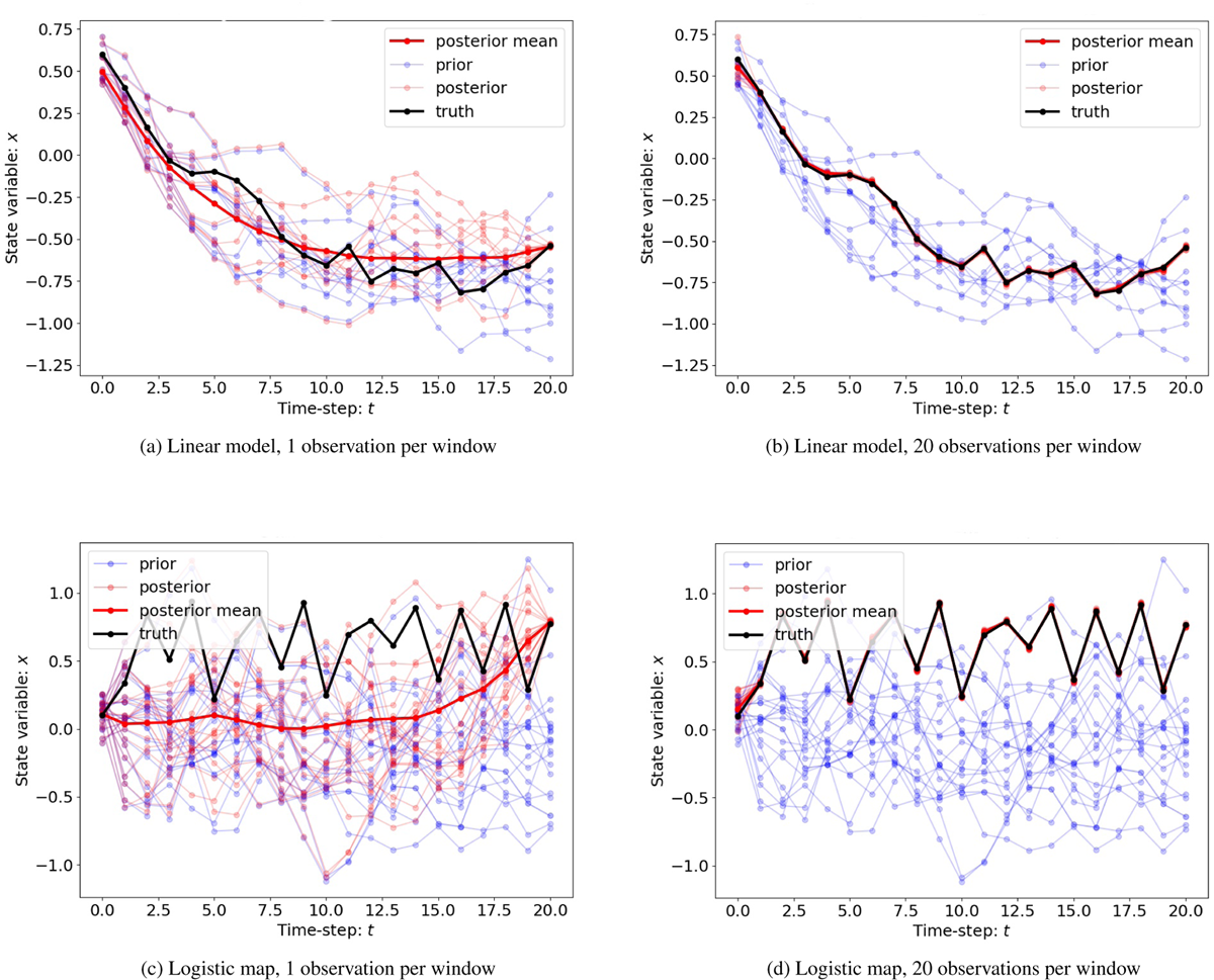
Figure 3
State update for both linear model and logistic map with different number of observations over a single simulation window using EnKS.
The top row of this figure shows the results with the linear model. In this case, the EnKS is capable of recovering an analysis mean quite close to the truth. The availability of more observations makes an important difference, as noted in the results shown in the two columns (left shows 1 observation per window, right shows 20 observations per window). In this simple linear case, even with very sparse observations, the EnKS can still provide a fair estimation of the state.
The bottom row shows the results with the logistic map. In the case with a single observation at the end of the simulation window, the EnKS was unsuccessful, which is expected considering the length of the assimilation window, and that joint estimation is being performed. To obtain a better results, more information from the observations is needed. With dense observations, observing every time-step for instance, the EnKS provides a correct estimation of all the state values at all time steps.
4.2 Parameter estimation in the linear model
4.2.1 One-parameter estimation
Our first experiments with the linear model consist of trying to estimate the parameter ω via the EnKS, using the one-parameter autocorrelation shown in Eq. (37). The results are shown in Figure 4. This figure has four panels. Panels (a), (b) and (c) have the same format, the difference amongst the panels is the number of observations per assimilation window. In each panel, the black vertical line shows the true value of the parameter. Different pdfs are displayed, computed as histograms using the ensemble members. The blue line shows the background pdf for the estimated parameter, whereas the orange-red lines correspond to the analysis pdfs after different number of assimilation windows. We see that the DA system works well for one-parameter estimation, especially with multiple observations. In fact, even with a single observation at the end of each simulation window, the analysis pdf moves towards the true ω, and the variance of the posterior pdfs is smaller than that of the prior, and it gets smaller as the number of consecutive assimilation windows increases. The effect of using more observations in each simulation window is to accelerate the convergence of the posterior pdf towards a stationary distribution. Panel (d) illustrates more clearly the evolution of the analysis estimator for sequential assimilation windows (in the horizontal axis). The blue horizontal line shows the value of the background mean , whereas the horizontal black line shows the true value of the parameter ωr = 0.5. In this case, we only track the analysis mean (solid colour lines) and the analysis standard deviation (shaded colour areas). With one observation at the end of the assimilation window, the convergence of the analysis mean is slow, taking about 50 assimilation windows before the analysis mean and standard deviation stabilise. There is, however, a considerable bias with respect to the true parameter. Increasing the number of observations in the assimilation window accelerates the convergence of the mean estimator. The cases with 5 and 20 observations per assimilation window approach their final value between 10 and 20 assimilation windows. The final estimate with 5 observations is still slightly larger than the true parameter. The estimate with 20 observations satisfactorily converges toward the real parameter from below, although at the end of the 80 assimilation windows a small gap still remains, much larger then the estimated uncertainty in the ensemble.
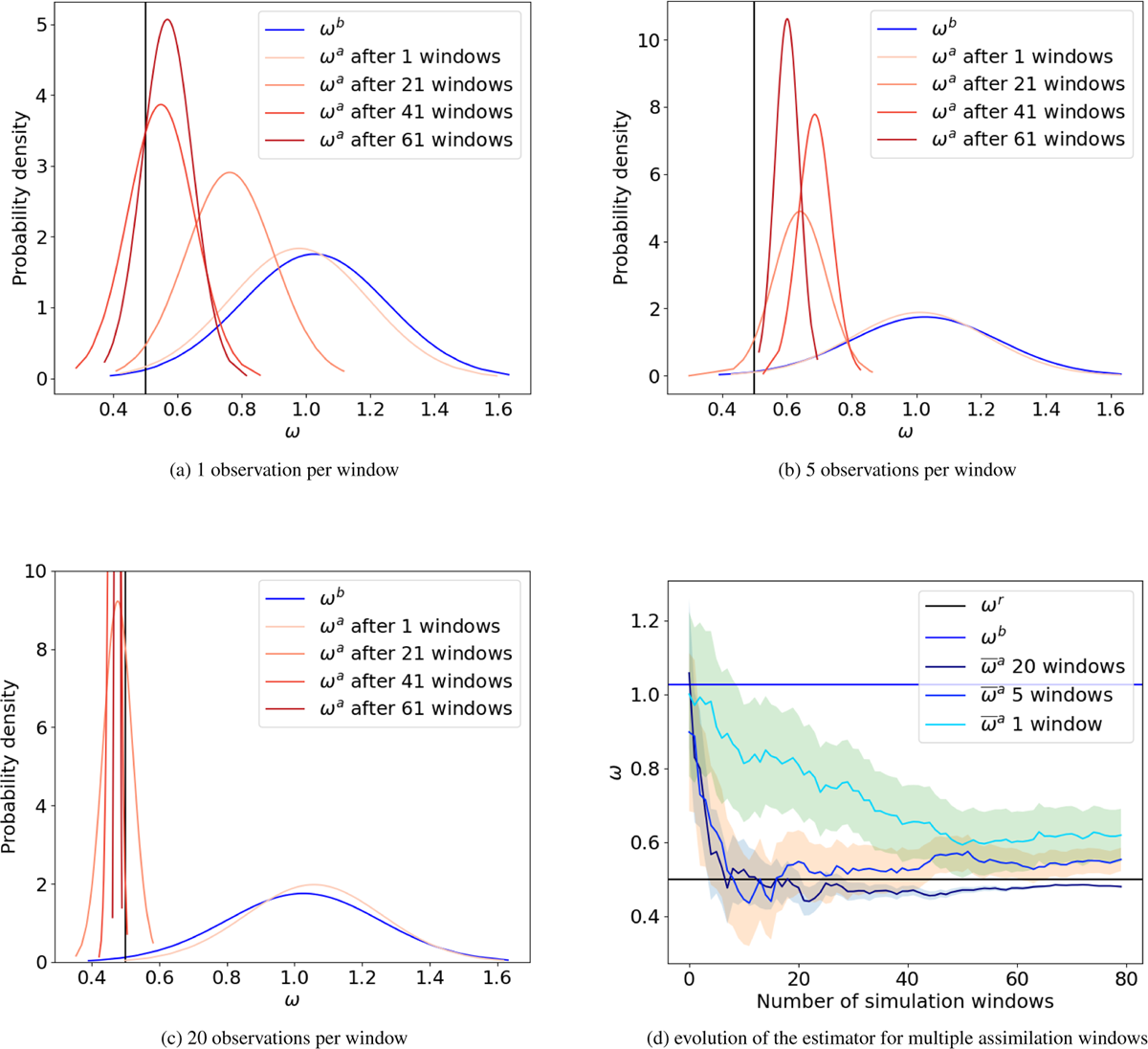
Figure 4
(a)∼(c) Exponential scale estimation with different numbers of observations and simulation windows using the EnKS and (d) the convergence of the mean of posterior pdf with the number of simulation windows.
We perform similar experiments with the IEnKS. Recall that in this case the number of iterations can influence the performance of the smoother. We analyse the effect of the number of iterations in Figure 5. This figure has two similar panels corresponding to 1 observation (left) and 20 observations (right) per window. The blue horizontal line denotes the background mean, and the black line the real parameter value. In each panel we plot several lines corresponding to analysis mean after different number of assimilation windows, as well as a shaded area corresponding to the analysis standard deviation. In the horizontal axis we have the number of iterations in each window. These iterations use a fixed step length δ. Perhaps the most important message of this figure is that the IEnKS results are independent of the number of assimilation windows since there is not a noticeable difference between the different lines. For one observation at the end of the assimilation window, the estimator has not fully converged after 20 iterations. It seems that at least 5 iterations per window are necessary for the IEnKS to show reasonable performance. In the case of 20 observations per window, it takes between 15 to 20 iterations for the IEnKS to converge to the true value of the parameter. Again, the number of assimilation windows does not matter. Based on these results we fix the number of iterations in the IEnKS to Niter = 10 for the rest of our experiments. In practice, one aims to perform as few iterations as possible to minimise computational expenses. We implement the IEnKS with a different numbers of observations and simulation windows. These results shown in Figure 6. The overall format of this figure is the same as that of Figure 4. Panels (a) to (c) reveal that the convergence to the analysis pdf is faster with more observations per window, and the resulting consecutive analysis pdf’s have smaller variance. Panel (d) reveals interesting results. For the three observation frequencies, the major changes to the analysis mean occur in the first 20 assimilation windows. For the cases with 1 and 5 observations per window, the bias in the final analysis mean is reduced considerably with respect to the estimators obtained by the EnKS. With 20 observations per window, the estimation is remarkably accurate, with the analysis mean oscillating around the real parameter value after 50 windows and remaining there.
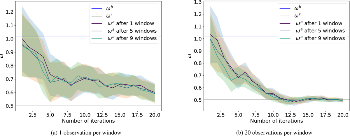
Figure 5
Analysis mean and standard deviation resulting from using IEnKS with different number of observations (panels), iterations (horizontal axis), after different number of simulation windows (lines).
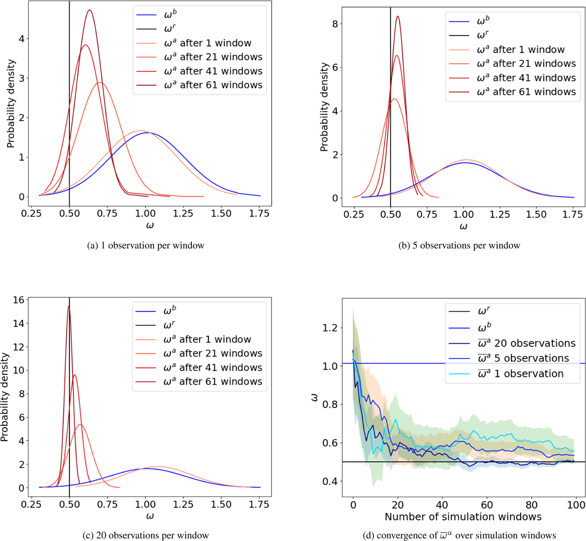
Figure 6
(a)∼(c) Exponential scale estimation with different numbers of observations observations and simulation windows using IEnKS and (d) the convergence of the mean of posterior pdf with the number of simulation windows.
In this subsection we have shown that EnKS converges to the real parameter value but a small bias remains, while its uncertainty estimate tends to contain that real value. The results show significant improvement increasing in the number of observations and the EnKS benefits from more assimilation windows. Next step is to extend our experiments to a more complex model error setting with two unknown parameters.
4.2.2 Two-parameter estimation
For this part of the experiments, we implement the model error with formulated in Eq. (39), which contains both decaying and oscillatory parameters. We start by experimenting with the EnKS. This method, however, fails to find the correct values for both parameters even in the case with observations every time step. This case is shown in Figure 7. This figure shows the background (blue line) and analysis (orange-red lines) pdf’s for the oscillatory (left) and decaying (right) parameters. The vertical black lines correspond the true parameter values. The figure illustrates how the mean of the analysis pdf converges towards wrong values of the parameters, with noticeable variance reduction after successive assimilation windows. This behaviour suggests that the minimisation process in the IEnKS is converging to an incorrect local minimum. To explore the failure of the EnKS in this case, it is useful to display the cost function of the problem. This requires computing Eq. (32) using Eq. (39) and Eq. (41). For simplicity, we do this for the case of a single operation at the end of the assimilation window. Before explaining the result, we need to recall some aspects of this function:
The input of this function is the vector u and the output is a scalar. The function maps 1 + τ + Nθ values into a single one.
The background elements needed by the cost function are the background mean and and covariance Du.
The observation elements needed by the cost function are the actual observation y and its variance r2.
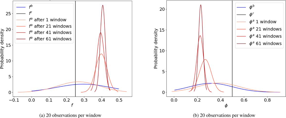
Figure 7
Two-parameter estimation, f (left) and φ (right), using the EnKS with 20 observations and different number of simulation windows.
In Figure 8 we start with a simple setting. We use the exact mean and covariance Du, as well as the observational variance r2 from section 3.3. Since we are not interested in the behaviour of the cost function with respect to the state variables, we set the state variables to a fixed value. and we only let the values θ = [f,φ]T vary freely. We plot a cross-section of the cost-function in the two-dimensional parameter space. We choose x0 = 0 and ε1 = … = ετ = 0.1 –note that we have to choose a value different from zero, otherwise the cost function would be blind to the variation in model error parameters.
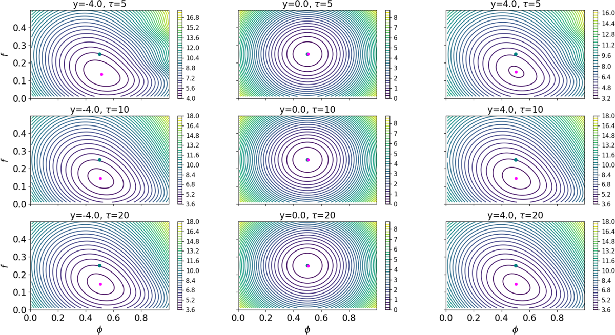
Figure 8
Exact cost function including the two-parameter model error, the state variable, observations with different number of time-steps and values of observations using the EnKS. The blue point represents the analysis value predicted after 1 EnKS step (with no extra iterations), and the pink point represents the exact global minimum.
Figure 8 has nine panels. Each one of the columns correspond to a different length of the assimilation window (recall that the observation is taken at the end), and each one of the columns correspond to a different given observation. We already know that the resulting cost function is not quadratic, and that the deformation from a quadratic cost function grows as the number of time step grows, and as the difference between the given observation and the predicted observation is larger. This is exactly what we observe in the figure. Both the first and third columns, when the observations are y  4.0 respectively, show the largest deformation of the cost function and this grows for the rows from top to bottom. The middle panel (y = 0) sees little deformation from a paraboloid. For each panel, the blue dot represents the background mean values of the parameters, and the pink dot corresponds to the global minimum of the cost function. In all cases, the cost function is still concave and there is a unique minimum to be found.
The simple case shown before is not what the EnKS encounters in practice. First of all, we do not know the real background covariance matrix, so this comes from a sample estimator. Second, the cost function is applied to each ensemble member separately, and therefore the background mean is just the background value for each member. The final analysis estimator is the mean of the Ne estimated minima. We explore this in Figure 9. First of all, we fix given observation to y = –4. Each column represents a different ensemble member (3 members out of the 200 we used to compute background statistics), and each row represents a different length of the assimilation window. To produce these cost functions, the background values are random realisations of the distributions for the initial conditions, model errors and parameter values shown in section 3.3. Again, we are interested in the behaviour in the two-dimensional parameter space, so we fix all the state variables to the same constants as before. What we see is very different from Figure 8. Figure 9 shows cost functions which are not convex, in fact they have very intricate topographic features such as narrow elongated ridges and valleys, and even some local mimima and maxima. The global cost minimum is difficult to converge to in a single application of the EnKS. In fact, this does not happen. We see that as the assimilation window length increases, the complicated features of the cost function increase. This agrees with the unsuccessful results we had seen in Figure 7. Therefore, it is necessary to apply a number of smaller steps via iterations in an IEnKS.
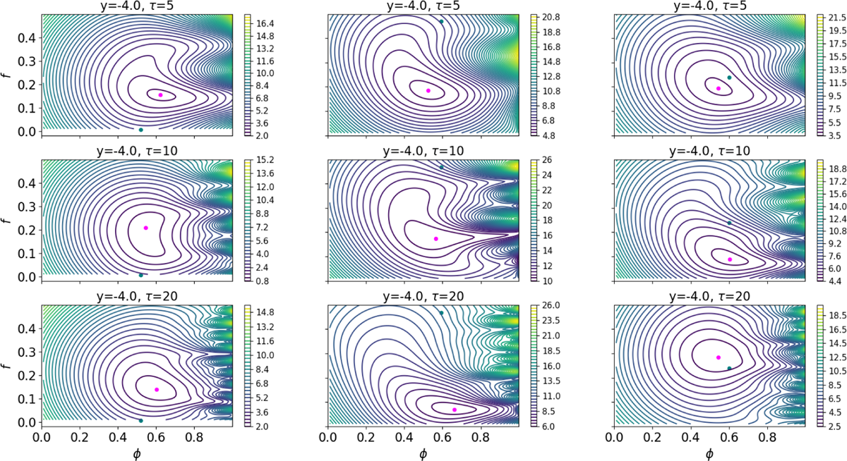
Figure 9
Sample cost function of different ensemble members (from left to right, Ne = 2,4,8) including the two-parameter model error, the state variable, observations with different number of time-steps and values of observations using the EnKS. The blue point represents the analysis value predicted after 1 ENKS step (with no iterations), and the pink point represents the exact global minimum.
We now apply the IEnKS to avoid getting stuck in a valley or a local minimum in the minimisation process. The results for the two-parameter estimation using IEnKS are shown in Figures 10 and 11. We apply the IEnKS with 10 iterations and a fixed step length δ = 0.3.
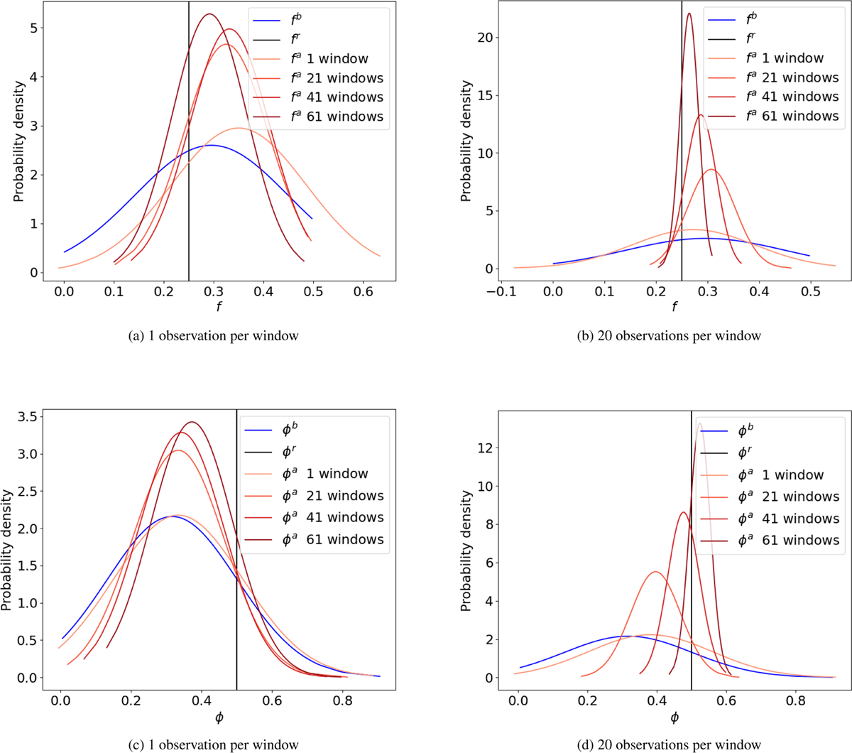
Figure 10
Two-parameter estimation using the IEnKS with different number of observations and simulation windows, and 10 iterations.
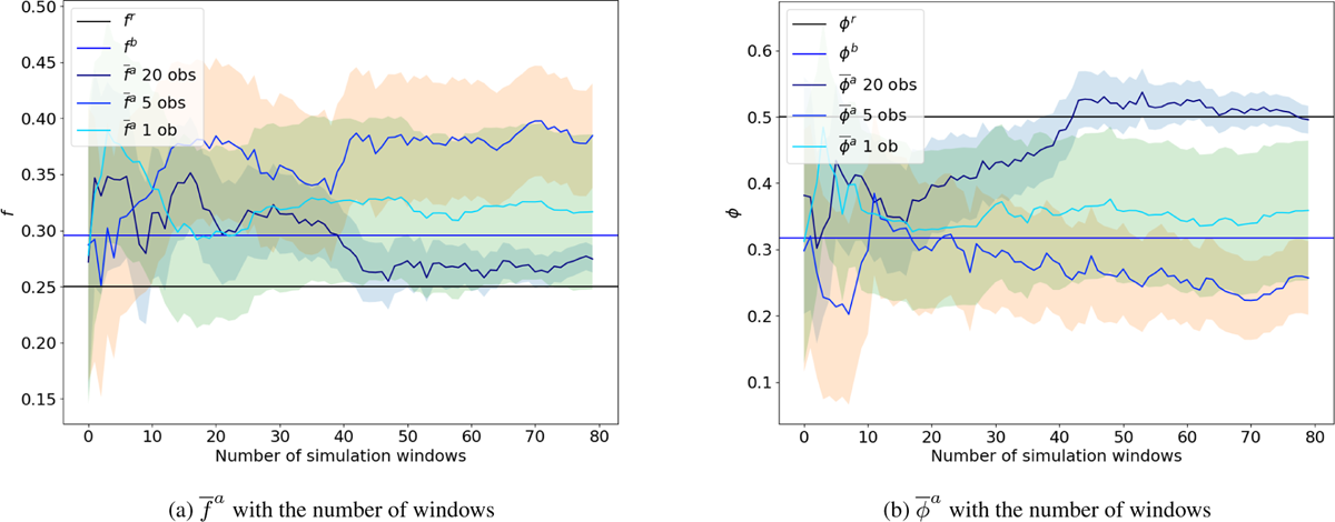
Figure 11
Posterior mean of the two parameters over the number of simulation windows with different number of observations.
Figure 10 shows the ensemble background and analysis pdfs (after different number of assimilation windows) for the oscillatory (top row) and decaying (bottom row) parameters, for 1 observation (top row) and 20 observations (bottom row). This figure reveals that the IEnKS works fairly well in this case. Similar to the results with the single parameter estimation, the two-parameter estimation results improve with the increase in the number of observations and assimilation windows in the simulation period. The IEnKS estimation converges towards the correct values of both parameters. In the case of only 1 observation in the assimilation window, the pdf stops short of the real value (black line), while in the case of 20 observations the estimation is better. Figure 11 tracks the evolution of the analysis mean and standard deviation for the two parameters (one for each panel) as the number of assimilation windows increases, and for three total number of observations: 1, 5 and 20. The true and background mean values are shown with horizontal lines, black and blue correspondingly. Note the improvement in the estimation as the number of observations increase. Even for observations every time step, there is a bias in the final estimation of the frequency parameter, while the decay parameter is captured in the ensemble uncertainty. Compared with the results from the one-parameter estimation, the two-parameter estimation problem seems to be much more complicated, and requires more observations to make the estimation work.
In closing the experiments for this subsection, we want to see how the IEnKS works with different initial guess for the two parameters. Given the complicated shape of the cost function, it is conceivable that we may get stuck in local minimums, even when using this sophisticated iterative method. We divide the two-dimensional parameter space into four quadrants, and we choose starting points in each one of the quadrants. These results are shown in Figure 12. This figure shows results in the case of one observation (left) and 20 observation (right). In both cases, the true values of the parameters are at the centre of the quadrants (denoted with a black dot). We see that the position of the initial condition can have serious impact on the estimation results. When we only observe at the end of the window most initial conditions do not lead to a value close to the true value. In fact, we see that the DA system cannot distinguish between parameter values lying roughly on a straight line defined by the red dots. On the other hand, when we have observations at every time-step, the posterior seems to get fairly close to the true values of the parameters, but many local minima exist around the true values. The results show the importance of the initial guess of the parameters on the parameter estimation results.
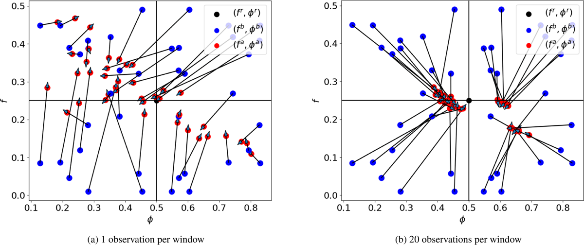
Figure 12
Two-parameter estimation for different priors using the IEnKS with different number of observations and simulation windows after 10 iterations. The blue dots show different background values, used as initial conditions for the minimisation. The red dots show the obtained analysis values. The black dot in the centre shows the true values for the parameters.
After experimenting with the linear model, our next step is extending the experiments of two-parameter model error autocorrelation to the nonlinear model, the logistic map.
4.3 Parameter estimation in a non-linear model
The last experiments we perform are also the most challenging. In this case our true model is the logistic map with the damping coefficient γ = 3.99, and the proxy model is linear model with auto-correlated model error. The true model error autocorrelation in this case has both an oscillatory and decaying behaviour (this can be diagnosed offline as described in section 3), so we directly try two-parameter estimation. Since the EnKS failed on the two-parameter estimation even with the linear model, we decide to only apply the IEnKS with 10 iterations, over times windows of 10 time steps long.
In our first experiments we try to estimate f and φ using the IEnKS with a fixed iteration step length δ = 0.3 as used in the linear experiments. The results of these experiments are shown in Figure 13 for both parameters (rows) and for 1 and 20 observations in the window (columns). With 1 observation at the end of the window the smoother does not seem to converge, and with 20 observations convergence seems to occur, but to incorrect values of the parameters. Increasing the number of iterations pr window or the number of windows did not improve results.
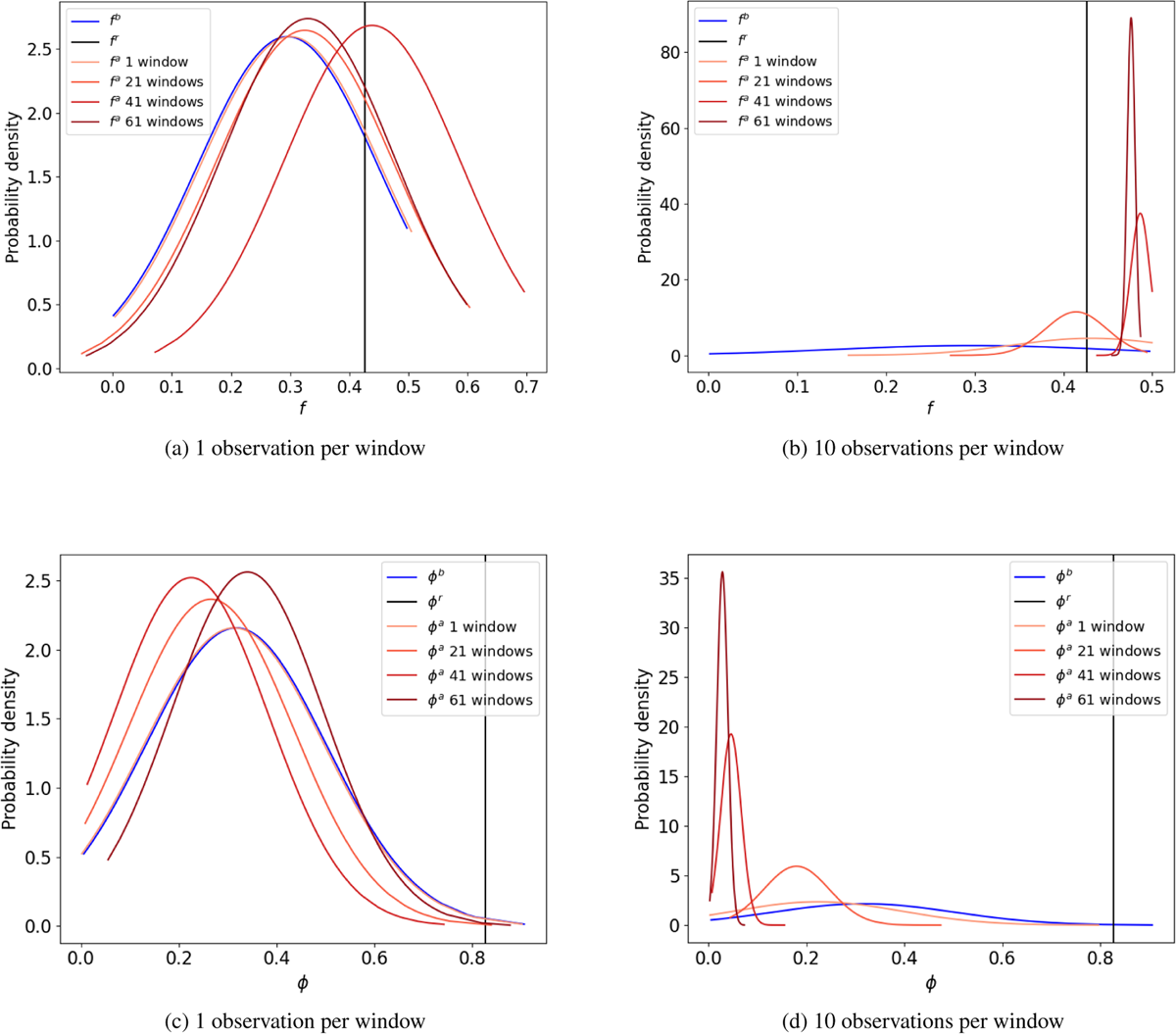
Figure 13
Two-parameter estimation using the IEnKS with the logistic map, using a fixed iteration step length (δ = 0.3), 10 iterations per window, different number of observations and simulation windows.
Since the IEnKS with a fixed step length δ fails to estimate the parameters directly, we explored three further experimental settings. In the first we transform the estimation problem to a more linear setting by estimating lag-1 and lag-2 autocorrelations of the model error (labelled as AC(1) and AC(2) respectively), and then transform the results to f and φ as the following:
In the second setting we use a decaying step length δ while using the untransformed parameters. However, Figure 14 shows that neither method is successful, suggesting that the problem is highly nonlinear and a more careful tuning of the minimization is required.
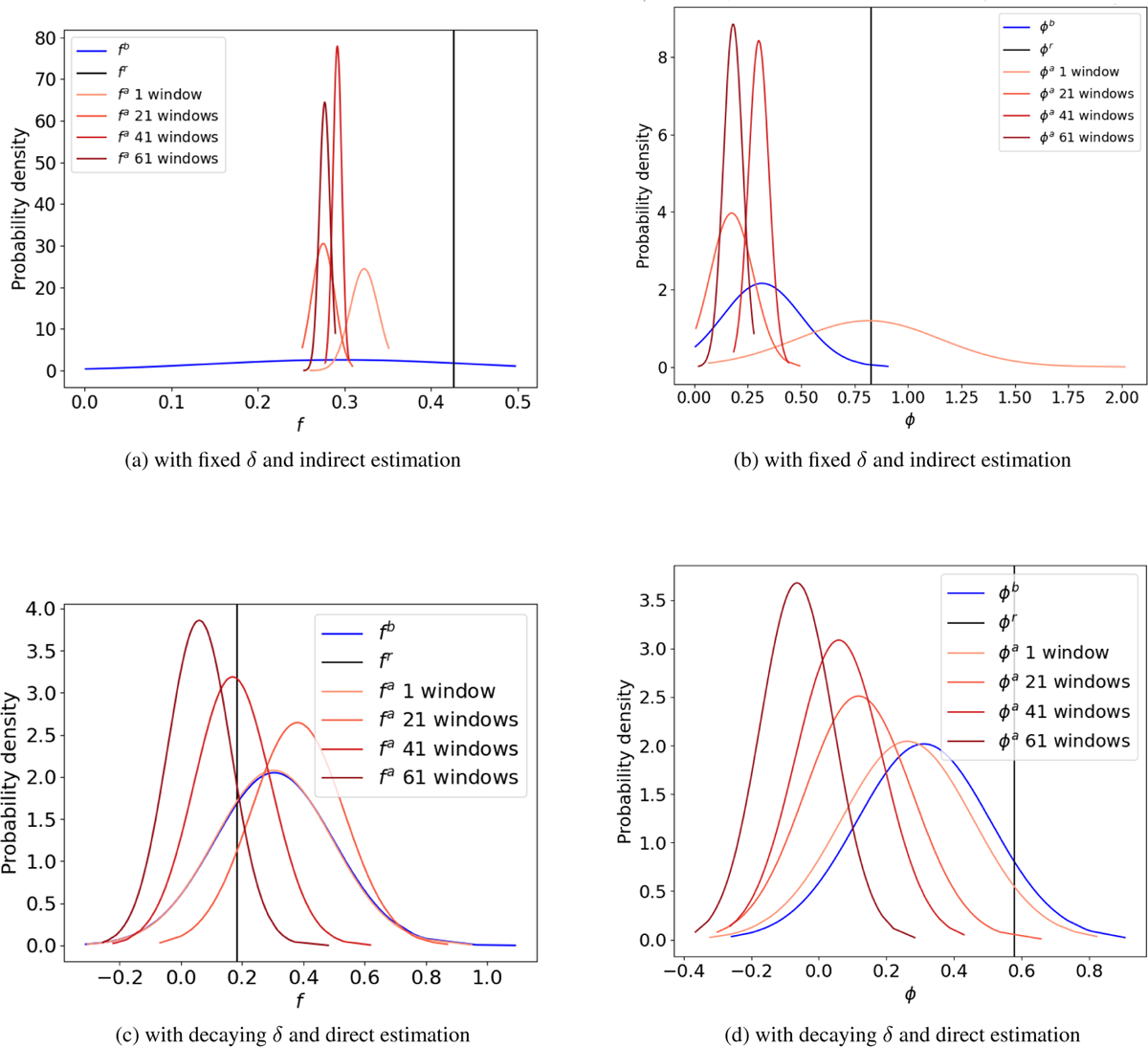
Figure 14
Two-parameter estimation using the IEnKS with 10 observations per window after 10 iterations with the logistic map. On the top panel, (a)∼(b) the iteration step-length is fixed (δ = 0.3), and we estimate the lag-1 and lag-2 autocorrelation then transform them to f and φ. On the bottom panel, (c)∼(d) the parameters are estimated directly with a decaying δ.
In the third setting we both transform problem to first estimating the autocorrelations and applying a decaying step length. However, with only 1 observation in the assimilation window the IEnKS failed, no matter what we tried. For a fully observed system with 10 observations per assimilation window successful results can be achieved. We show results for reducing the step length δ by 2% after each iteration (i.e. c = 0.98 in Eq. (36)). From the two top plots in Figure 15, we can see that the results are similar to the successful results for the linear model shown in Figure 10. The posterior shows improvement with more simulation windows, and the variance decreases with more windows as well. Figures 15 (c) and (d) show that the posterior mean moves towards the right values for both parameters, with slowly decaying uncertainty.
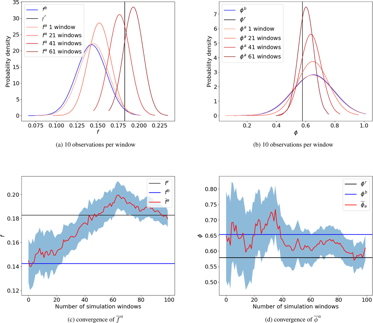
Figure 15
Lag-1 and lag-2 autocorrelation are estimated and transform to the parameters (a) f and (b) φ, using the IEnKS with a decaying iteration step length, 10 iterations per window, for different numbers of assimilation windows with the logistic map. The bottom two figures show the convergence of the posterior mean of (c) f and (d) φ over the number of simulation windows with observations every time-step.
Even though the minimization is successful the convergence is extremely slow, even in this simple zero-dimensional model. This illustrates that estimating parameters in model errors that are related to temporal correlations is a very hard problem.
5 Summary and conclusions
Including the model error in the DA process is a difficult task to tackle, especially when this model error possesses spacial and temporal correlation. The objective of this work is to test whether it is possible to include the estimation of time-related model error parameters in the DA process. We have shown that even in the case of linear dynamics, the model error parameters are involved in an intricate and non-linear way in the model evolution. We have therefore focused in the use of the EnKS and the IEnKS combined with parameter augmentation to solve the joint state-parameter estimation problem.
With a simple linear-regressive model and exponential decaying memory in the model error, the EnKS works well using the state augmentation method to estimate a single model error parameter, even with only one observation at the end of the assimilation window. The estimation results are improving with an increasing number of observations in each window, and by iterating over more assimilation windows. The IEnKS with 10 iterations gives slightly superior results compared to the EnKS in this case, as expected.
When the complexity of the temporal correlation in the model error is increased by including an oscillatory component state augmentation with the EnKS fails. Indeed, the cost functions involved show highly irregular shapes and convergence in one step is not possible. An IEnKS with a fixed iteration step length is shown to converge to the correct values when the number of observations in an assimilation window is high enough. The failure to converge with one observation at the end of the assimilation window can be traced back to the long valley with minimal gradients in the cost function, identified via different first guess values. There just isn’t enough information to estimate both model error parameters. However, we do see that the uncertainty in the estimates remains large, so the IEnKS does show consistent results. Increasing the number of observations in the window solves this problem.
The nonlinear logistic map proves to be more challenging when estimating both model error parameters. The EnKS always fails, and the IEnKF fails with the standard fixed step length and direct estimation of the parameters. The combination of a step length that decreases with iteration and transforming the problem by first estimating the autocorrelations in the model error solves this problem, although we need a fully observed system, and convergence is very slow.
Overall, we conclude that estimating temporal-correlation related parameters in model errors is a highly nonlinear problem, and more difficult than expected even in zero-dimensional systems. The number of observations in an assimilation window needs to be high enough for the smoother to have enough information on these parameters, and for nonlinear models careful tuning of an IEnKS is needed. The bottom line is that it is very well possible that the data-assimilation system does not have enough information to pinpoint the exact model error parameters, while at the same time we should realize that these parameterizations of model errors are approximate by their very nature.
It is important to keep in mind that these results were obtained with a very large ensemble size of 200 for a zero-dimensional system and two parameters. This choice made sense for the focus of this paper, but in reality the limited ensemble size will give rise to extra noise in the estimates. The IEnKS, while being a very powerful method, does not converge to the posterior pdf with growing ensemble size for nonlinear data-assimilation problems (see e.g. Evensen, 2018). Especially when multiple modes are present in the posterior, as in our case, several of the modes can be missed. This is problematic when local modes are almost as high as the global mode, in which case the correct solution to the data-assimilation problem is this family of modes. To find these fully nonlinear methods like local particle filters or particle flows are needed (see e.g. Van Leeuwen et al., 2019; Hu and Van Leeuwen, 2021; Evensen, Vossepoel, and Leeuwen, 2022).
Our next step is to investigate how these results carry over to more realistic and complex models such as a two-layer quasi-geostrophic model. The challenge in this case is whether the spatiotemporal model error correlation is separable or not. The ultimate goal is to have a online update for the model error within an operational system.
Funding Information
UK National Centre for Earth Observation (NCEO) and European Research Council via the EU Horizon 2020 framework under the CUNDA project with grant number 694509.
Competing Interests
The authors have no competing interests to declare.