
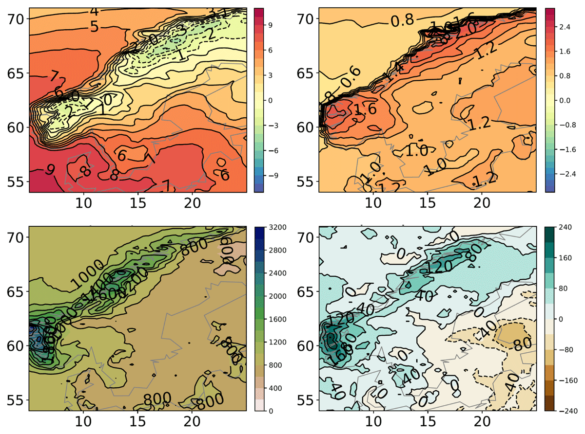
Figure 1
Annual mean temperature (°C; 1st row) and precipitation (mm; 2nd row) in the Scandinavian area for 1961–1990 (left) and changes between 1991–2020 and 1961–1990 (right). Data are taken from the reanalysis ERA5.
Table 1
Mean temperature (°C) and precipitation (mm) in Sweden from SMHIs climate indicators. Interannual variability is given as one standard deviation for temperature and as the standard deviation normalised with the mean for precipitation to give the coefficient of variation (CV that is given in %).
| NORMAL PERIOD | SEASON | TEMPERATURE | PRECIPITATION | ||
|---|---|---|---|---|---|
| MEAN ± 1 Σ | MIN/MAX | MEAN ± CV | MIN/MAX | ||
| 1961–1990 | DJF | –4.6 ± 2.6 | –9.5/–0.5 | 133 ± 26 | 72/203 |
| MAM | 3.2 ± 1.1 | 1.4/5.9 | 115 ± 26 | 49/158 | |
| JJA | 14.6 ± 0.8 | 12.7/16.1 | 203 ± 20 | 122/285 | |
| SON | 5.6 ± 0.9 | 3.5/7.9 | 193 ± 17 | 129/267 | |
| 1991–2020 | DJF | –2.8 ± 2.0 | –6.9/0.9 | 148 ± 23 | 47/195 |
| MAM | 4.4 ± 1.0 | 2.5/5.9 | 120 ± 20 | 84/174 | |
| JJA | 15.4 ± 1.0 | 13.3/17.3 | 229 ± 17 | 153/309 | |
| SON | 6.3 ± 1.2 | 3.9/8.2 | 188 ± 18 | 139/269 | |
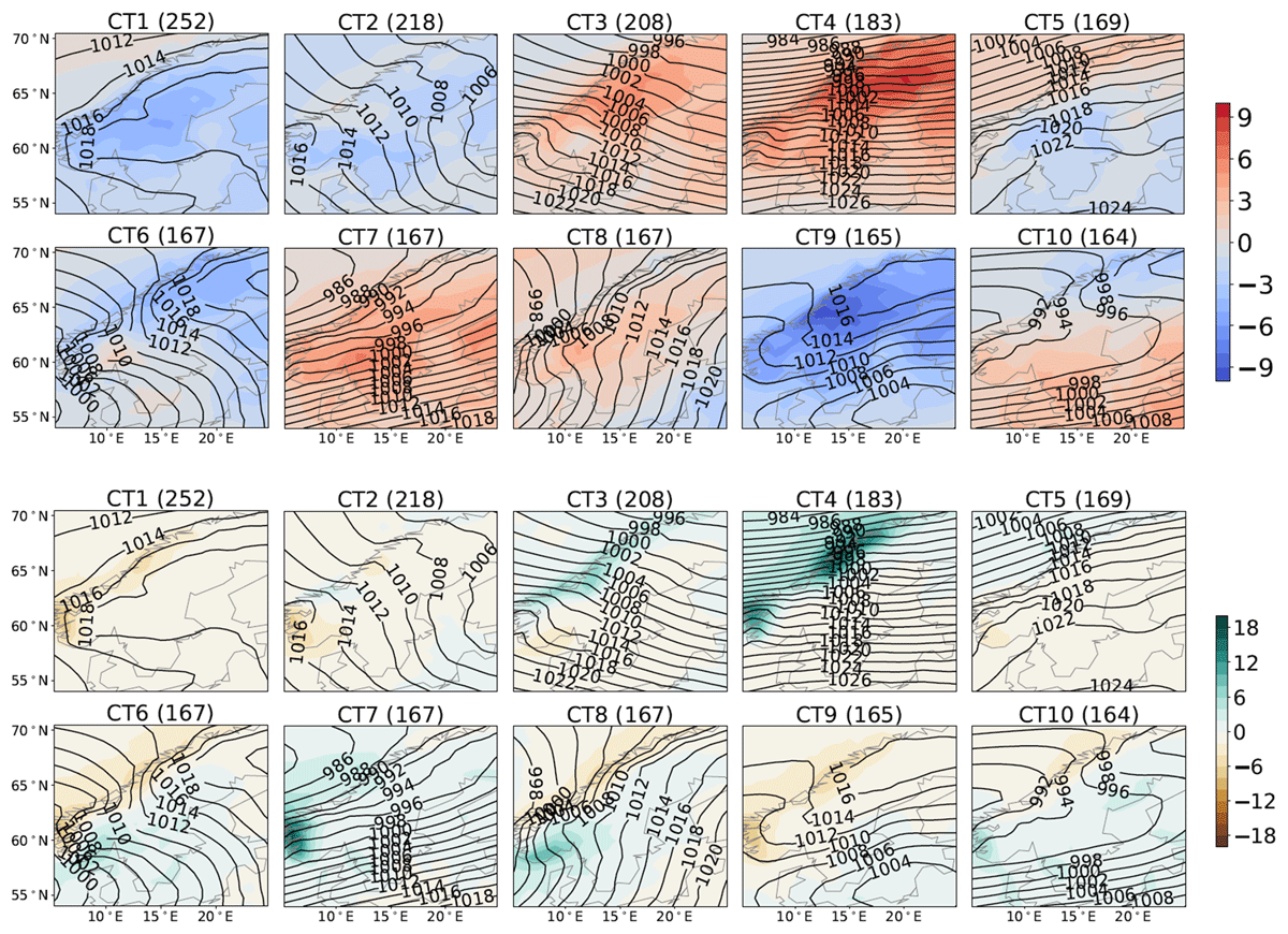
Figure 2
Ten circulation types generated using the SANDRA CTC method for all January days in 1961–2020. The frequency for each cluster is indicated as the number of days (out of a total of 1860) on top of each map. The isolines show composite averages mean sea level pressure. The colour shaded fields show corresponding temperature and precipitation anomalies relative to the monthly mean for temperature (top, °C) and precipitation (bottom, mm).
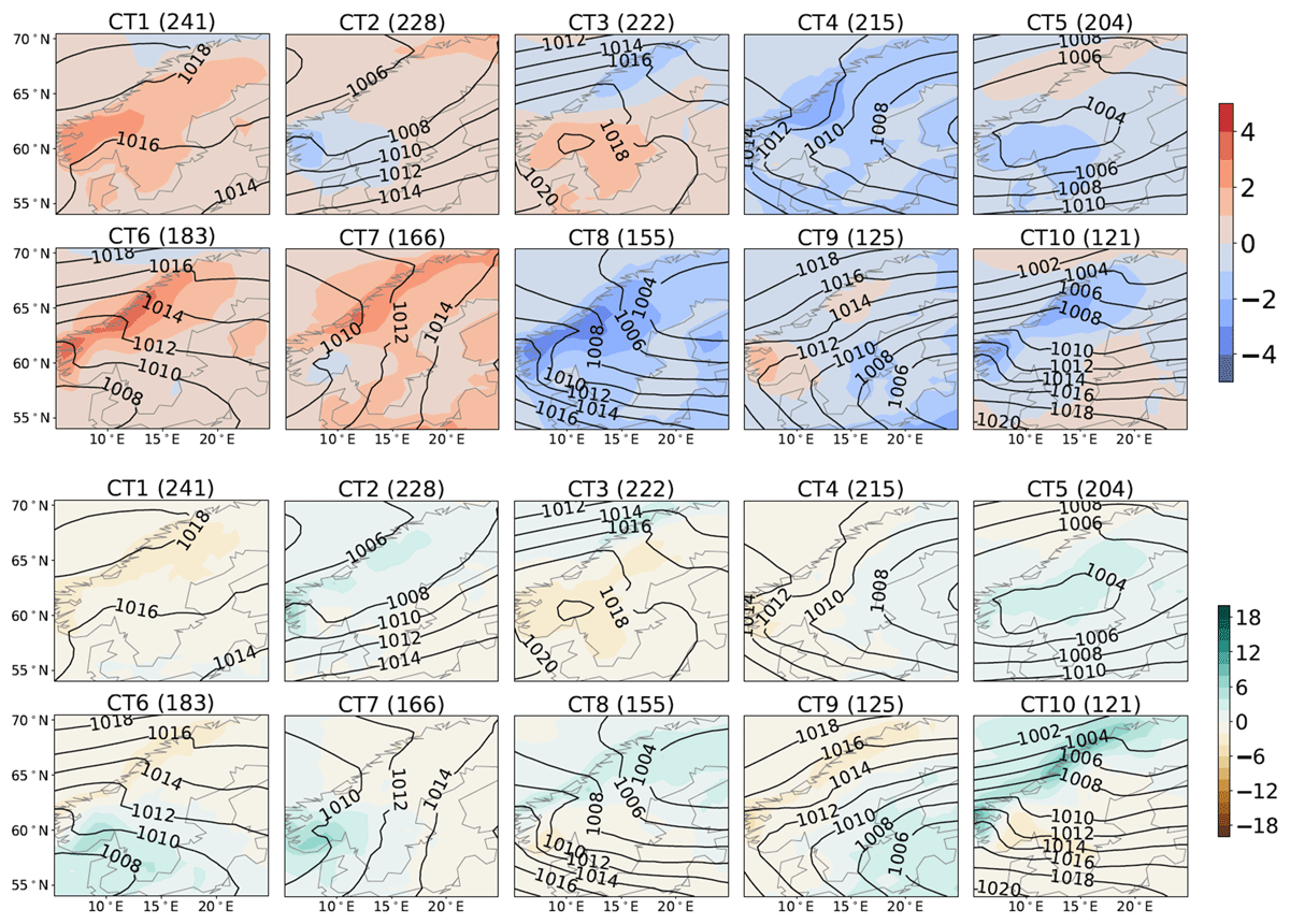
Figure 3
As Figure 2, except for July.
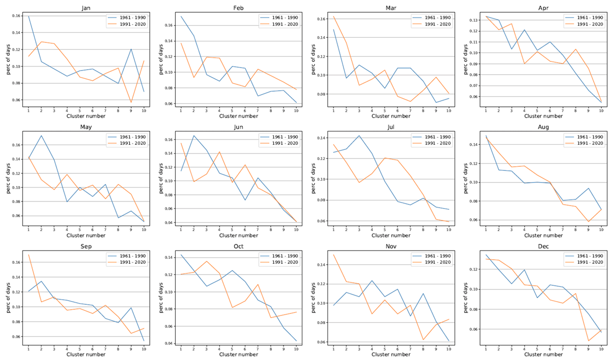
Figure 4
Frequencies for each circulation type in the two periods for 1961–1990 (blue) and 1991–2020 (orange). Note that circulation types are defined separately for each month and that it is not meaningful to compare the individual circulation type numbers between months.
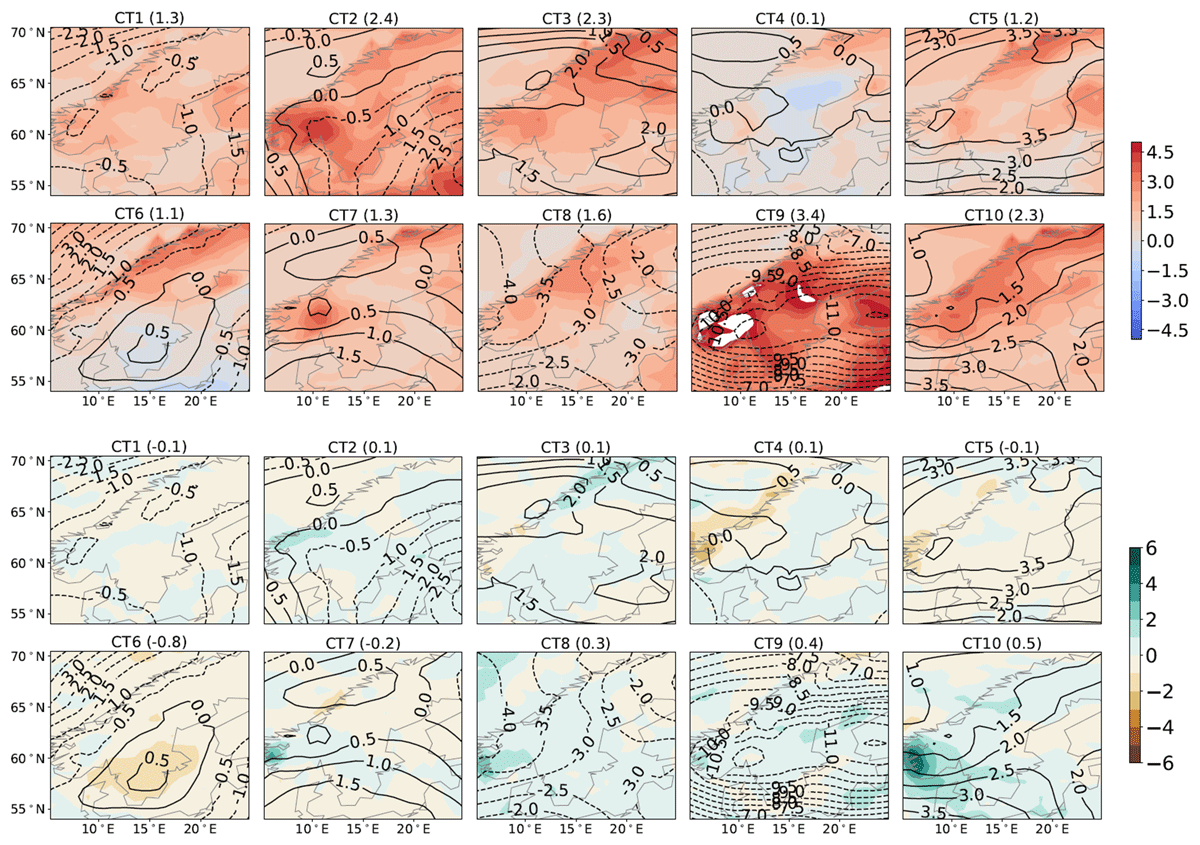
Figure 5
Difference for each circulation type in January (cf. Figure 2) between 1961–1990 and 1991–2020. The isolines show average change in mean sea level pressure. The colour shaded fields show corresponding changes in temperature (top, °C) and precipitation (bottom, mm). The numbers given on top of the panels are the average changes over Sweden between the two periods.
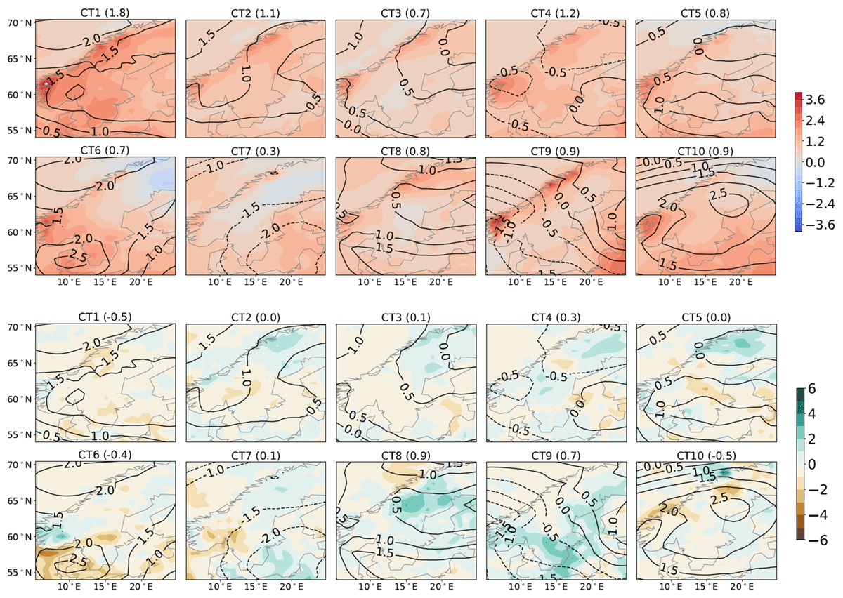
Figure 6
Table 2
Area average mean temperature change (°C) for Sweden between 1961–1990 and 1991–2020 for each cluster calculated from ERA5 data. Clusters for which the interquartile range of daily data changes by more than 0.5°C are marked with italics for decreased range and bold face for increased range. The rightmost column shows the corresponding northern hemisphere average warming according to HadCRUT5.
| 1 | 2 | 3 | 4 | 5 | 6 | 7 | 8 | 9 | 10 | NH | |
|---|---|---|---|---|---|---|---|---|---|---|---|
| JAN | 1.3 | 2.4 | 2.3 | 0.1 | 1.2 | 1.1 | 1.3 | 1.6 | 3.4 | 2.3 | 0.74 |
| FEB | 1.5 | 0.7 | 3.3 | 1.1 | 0.5 | 0.1 | 0.0 | 2.8 | 1.9 | 0.7 | 0.80 |
| MAR | 1.8 | 1.5 | 0.8 | 0.5 | 2.1 | 0.8 | 0.7 | 0.6 | 0.8 | 1.5 | 0.78 |
| APR | 1.3 | 1.6 | 1.2 | 1.3 | 1.6 | 1.5 | 0.8 | 1.0 | 0.5 | 1.0 | 0.77 |
| MAY | 1.0 | –0.2 | 0.6 | 0.7 | 0.5 | 1.4 | 2.2 | –0.1 | 0.3 | –0.1 | 0.66 |
| JUN | 0.6 | –0.3 | 0.1 | –0.2 | 0.3 | 0.1 | 0.1 | 0.0 | 0.6 | 0.4 | 0.66 |
| JUL | 1.8 | 1.1 | 0.7 | 1.2 | 0.8 | 0.7 | 0.3 | 0.8 | 0.9 | 0.9 | 0.65 |
| AUG | 0.8 | 1.5 | 0.5 | 0.9 | 1.2 | 1.1 | 1.0 | 0.8 | 0.4 | 0.9 | 0.68 |
| SEP | 0.5 | 1.1 | 1.1 | 1.5 | 0.7 | 0.7 | 0.4 | 1.0 | 1.9 | 0.5 | 0.67 |
| OCT | 0.4 | 0.9 | –0.4 | 0.9 | –0.8 | 0.3 | 0.2 | 0.3 | –0.4 | 0.3 | 0.74 |
| NOV | 1.5 | 1.1 | 1.1 | 2.5 | 1.6 | 0.8 | 0.6 | 1.0 | 0.3 | 1.7 | 0.76 |
| DEC | 2.8 | 0.9 | 0.2 | 2.8 | 1.6 | 2.1 | 2.6 | 1.9 | 0.7 | 1.7 | 0.70 |
Table 3
Area average mean change in precipitation intensity (%) for Sweden between 1961–1990 and 1991–2020 for each cluster and total for each month. Clusters for which the coefficient of variability (CV) of daily data changes by more than 10% are marked with italics for decreased range and bold face for increased range.
| 1 | 2 | 3 | 4 | 5 | 6 | 7 | 8 | 9 | 10 | TOTAL | |
|---|---|---|---|---|---|---|---|---|---|---|---|
| JAN | –14 | 9 | 7 | 5 | –14 | –27 | –5 | 14 | 37 | 18 | 8 |
| FEB | –11 | –10 | 7 | 0 | –11 | –18 | –1 | 16 | 0 | 28 | 7 |
| MAR | 8 | –39 | –15 | 19 | –12 | 10 | 6 | 2 | 0 | –2 | –7 |
| APR | –26 | –13 | –11 | –7 | –5 | –4 | –12 | –3 | 27 | 7 | –6 |
| MAY | 17 | 46 | 3 | 13 | 33 | 25 | 1 | 11 | 25 | 17 | 15 |
| JUN | –3 | 46 | 29 | 38 | 35 | 28 | 3 | 23 | 37 | 16 | 29 |
| JUL | –32 | 1 | 7 | 10 | 0 | –12 | 5 | 24 | 25 | –16 | 5 |
| AUG | 18 | 17 | –3 | 11 | –22 | 7 | 4 | 18 | 5 | 12 | 5 |
| SEP | –41 | 8 | –51 | 0 | 4 | 7 | –27 | –8 | 41 | –11 | –10 |
| OCT | 6 | 6 | –4 | –8 | 6 | –4 | 61 | 14 | –10 | –47 | 1 |
| NOV | –3 | –21 | –12 | –13 | –7 | –3 | –12 | 10 | –3 | 7 | –4 |
| DEC | –2 | –10 | 1 | 19 | 12 | –11 | 24 | 13 | 3 | –16 | 1 |
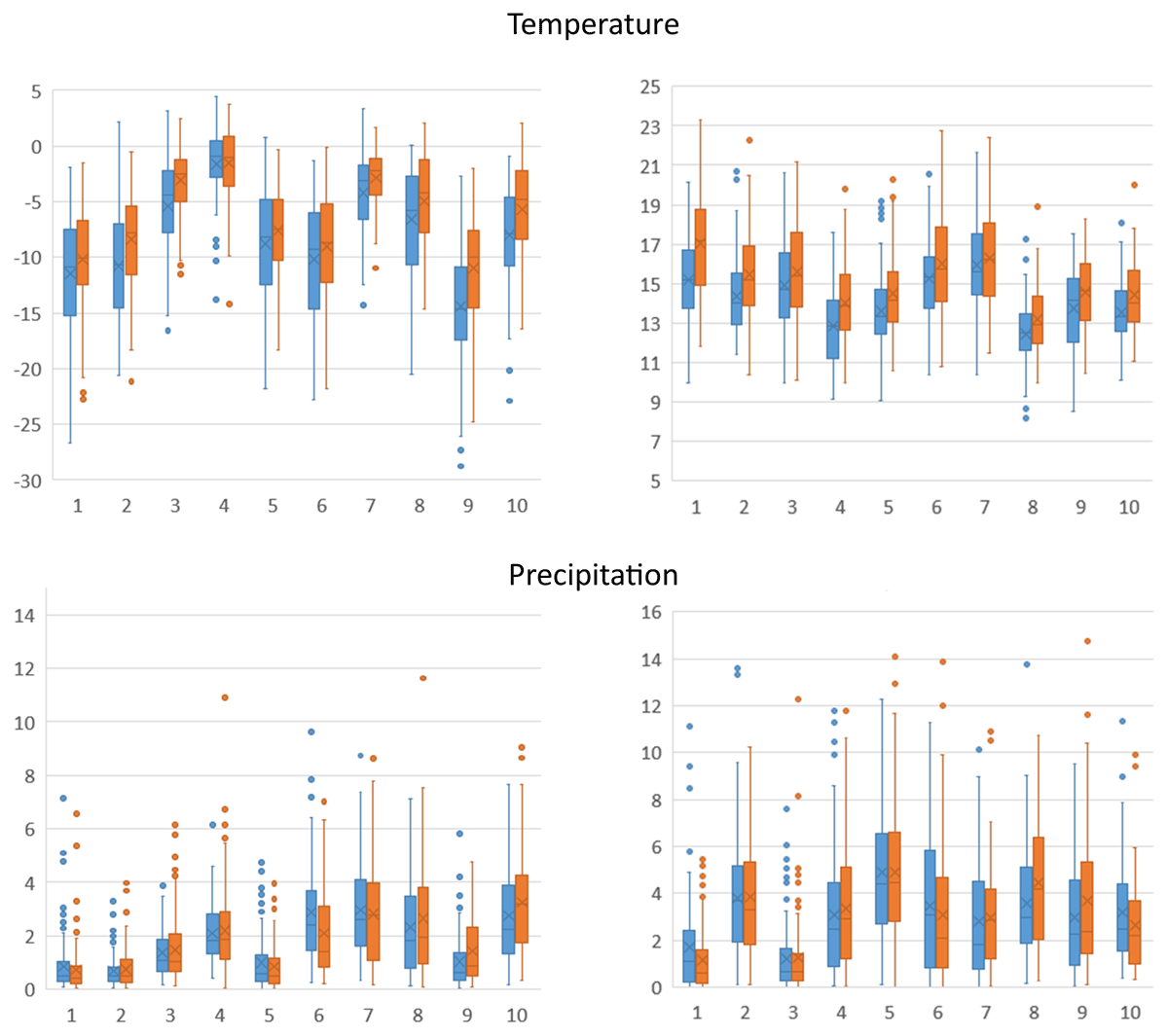
Figure 7
Distributions of daily data for the ten circulation types in January (left) and July (right). For each circulation type the blue boxplot represents 1961–1990 and the orange 1991–2020. The boxplots show the mean value represented with an x, the median represented by the central horizontal line, the 25th and 75th percentiles represented by the box. Points outside of 1.5 times the interquartile range from the respective 25th and 75th percentiles are considered to be outliers and are denoted by a point. The length of the whiskers is defined as the largest or smallest value not being an outlier. Units: °C for temperature and mm for precipitation.
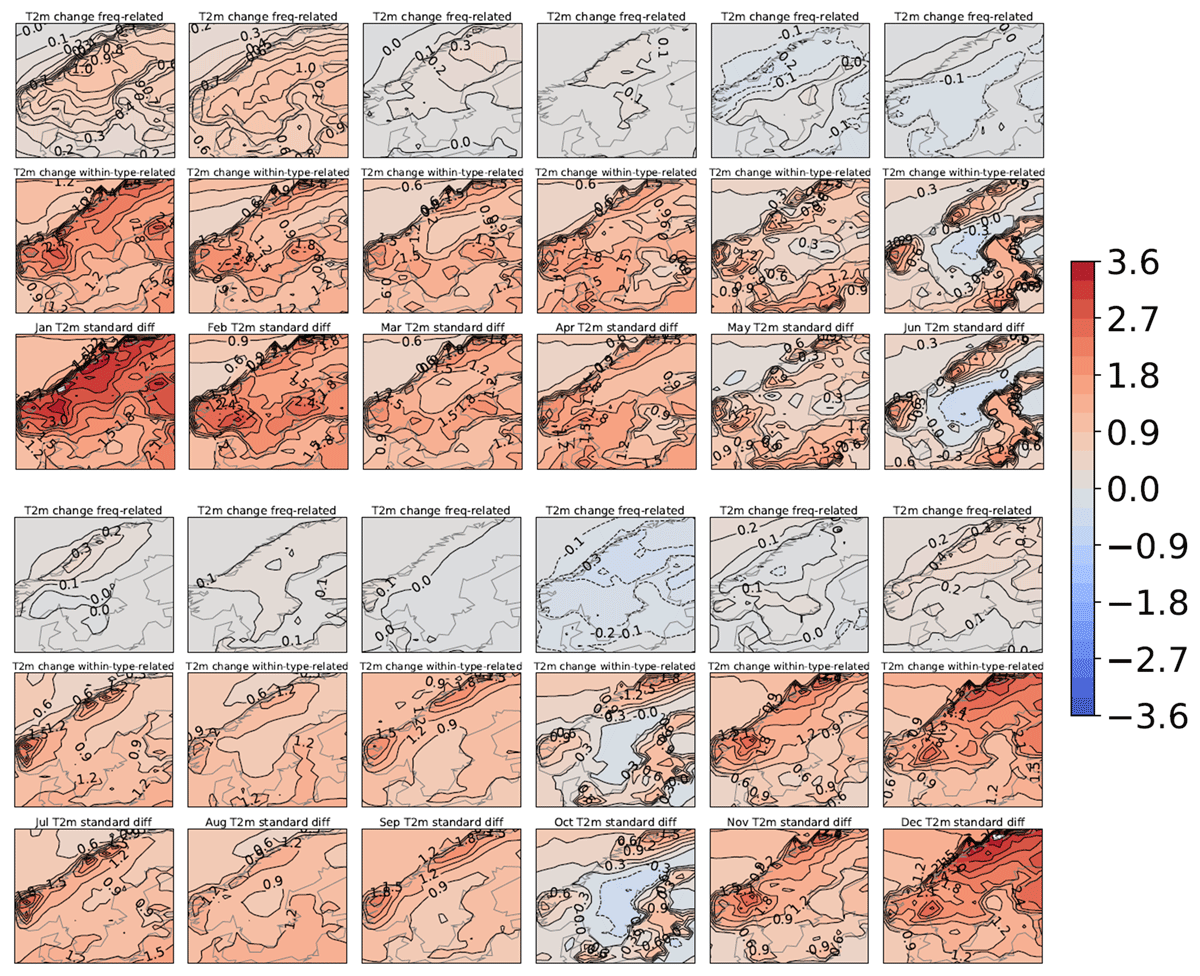
Figure 8
Temperature difference between 1961–1990 and 1991–2020 for January-June (upper part) and July-December (lower). The uppermost row for each month shows the difference that is due to changing frequencies of circulation types. The middle row shows the within-circulation type amplitude changes. The lowermost row shows the total changes. Units: °C.
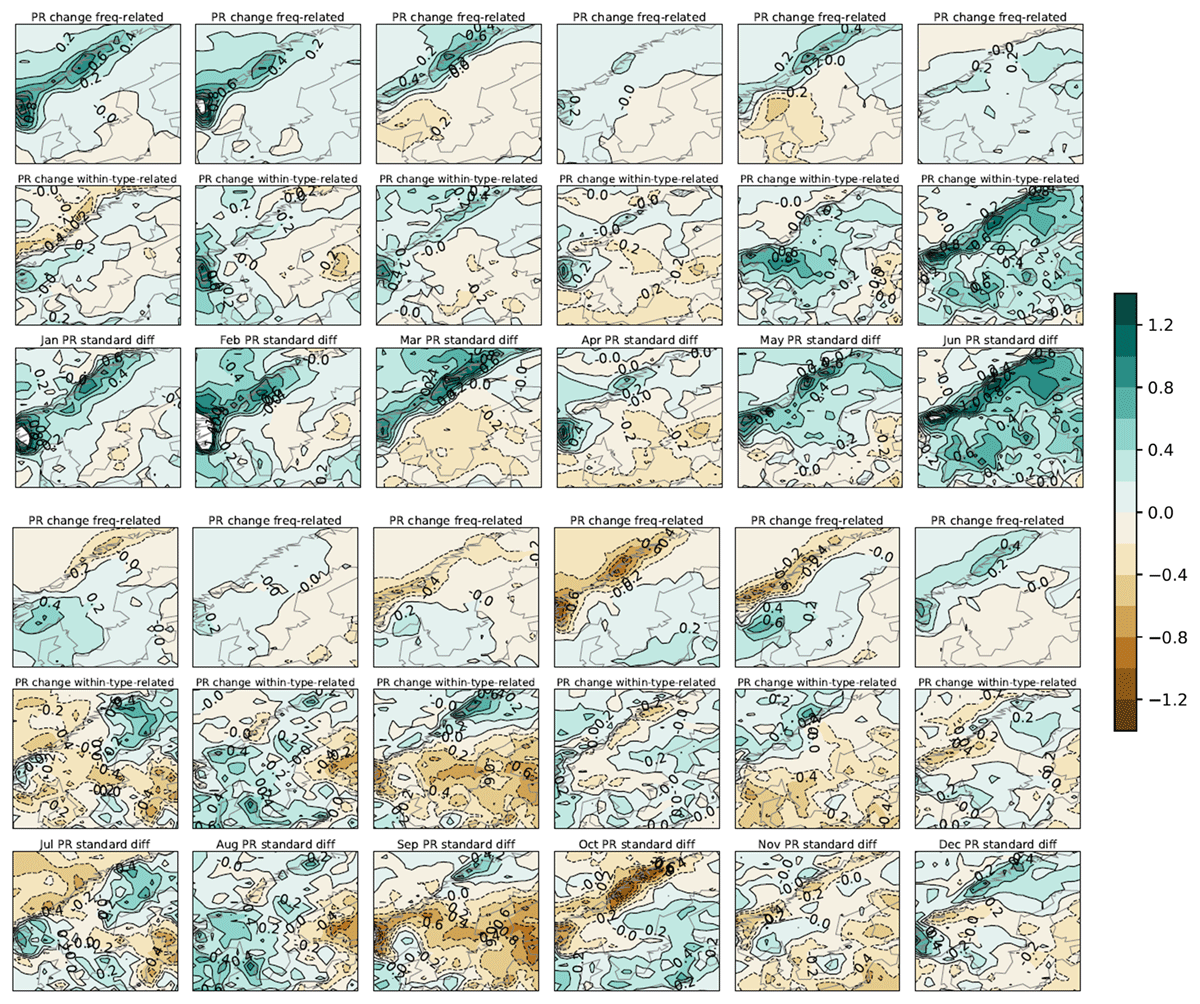
Figure 9
As Figure 8, except for precipitation. Units: mm/day.
Table 4
30-year average NAO-index and results from linear fits with temperature (T) and precipitation (PR) from the Swedish average derived from the SMHI stations. The linear fits are done separately over the two 30-year periods. The regression coefficients (r2), slopes (k) and intercepts (l) are given.
| NORMAL PERIOD | SEASON | NAO | R2 | K | L | |||
|---|---|---|---|---|---|---|---|---|
| T | PR | T | PR | T | PR | |||
| 1961–1990 | DJF | –0.25 | 0.59 | 0.17 | 1.70 | 11.7 | –4.22 | 136 |
| MAM | 0.02 | 0.38 | 0.04 | 1.17 | 10.5 | 3.18 | 114 | |
| JJA | 0.13 | 0.09 | 0.02 | 0.74 | –17.6 | 14.5 | 205 | |
| SON | 0.07 | 0.35 | 0.00 | 1.00 | 0.23 | 5.51 | 193 | |
| 1991–2020 | DJF | 0.37 | 0.61 | 0.24 | 1.38 | 14.9 | –3.31 | 143 |
| MAM | 0.13 | 0.46 | 0.02 | 0.99 | 4.92 | 4.29 | 119 | |
| JJA | –0.08 | 0.03 | 0.21 | 0.42 | –42.9 | 15.5 | 226 | |
| SON | –0.10 | 0.28 | 0.02 | 1.39 | 10.9 | 6.39 | 189 | |
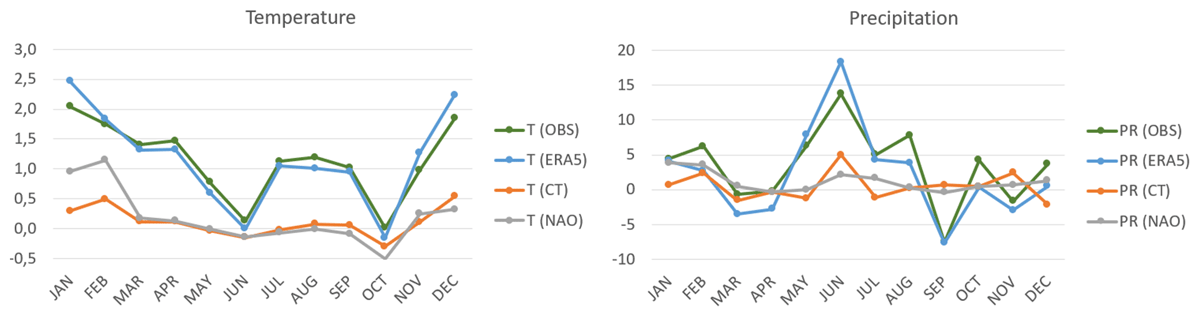
Figure 10
Changes in Swedish mean temperature (left, °C) and precipitation (right, mm/month) between 1961–1990 and 1991–2020. Observations (green) are from the SMHI data, reanalysis (blue) from ERA5. The synthetic temperature and precipitation series are derived from changes in the NAO-index (grey) and the analysis of circulation types (orange). See text.