
Introduction
In order to predict accurately the atmospheric state evolution, Numerical Weather Prediction (NWP) models require a realistic representation of the atmosphere at initial state. This is particularly true in the lower part of the troposphere for the description of the surface and the boundary layer, where important vertical energy, water and momentum exchanges take place. The initialisation of the surface and atmospheric parts are done by data assimilation. The developments of space-borne instruments have improved the surface and atmosphere observation capabilities and allowed NWP models to assimilate more data with higher frequency and coverage (Montmerle et al., 2007). At Météo-France, the convective-scale limited-area model AROME (Applications of Research to Operations at Meso-scalE) assimilates both conventionnal and satellite observations to initialize the state of the atmosphere at each analysis time every hour, with a large part of radar observations. For the representation of surface fluxes and exchanges with the atmosphere, AROME model is coupled to the surface modelling platform SURFEX (Externalized Surface) (Masson et al., 2013).
In NWP models, the assimilation of satellite data requires the knowledge of the atmospheric state and an accurate description of surface conditions, in particular of surface parameters such as surface temperature and emissivity. These surface parameters are used in the simulation of the model equivalent of the satellite radiances. However surface models can present deficiencies and a possible approach, used at Météo-France, to obtain realistic surface conditions in the radiance simulation, consists in retrieving one of these parameters for each sensor using a channel located in an atmospheric window. This retrieved temperature or emissivity is then used for the simulation and the assimilation of the other channels of the instrument in the AROME model. For the assimilation of microwave sensors, the surface emissivity is retrieved (Karbou et al., 2006), since it has a larger range of variation than in the infrared spectrum, and a 1% error in the emissivity induces a 1 K error in the brightness temperature (Vincensini, 2013). For infrared sensors, the surface emissivity, which has less variability than in the microwave spectrum, is obtained from an atlas and the surface temperature is retrieved instead (Guedj et al., 2011) and (Boukachaba et al., 2015). However, this retrieved quantity is not used further in the surface analysis, no correction nor improvement of the surface temperature of the model is performed and the retrieval is computed at each analysis time.
NWP centers, including Météo-France, have used in-situ observations of screen level parameters to analyse soil temperature and moisture for several decades (Mahfouf et al., 2009), (Douville et al., 2000) and (Drusch and Viterbo, 2007). However the surface observation network is heterogeneous over the globe and there is a lack of observations over some regions. The assimilation of satellite observations, especially of ASCAT ((De Rosnay et al., 2013) and (Lindskog et al., 2019)) or SMOS ((Muñoz-Sabater et al., 2019) and (De Lannoy and Reichle, 2016)) surface soil moisture has been shown beneficial over such regions. Concerning surface temperature, several studies have already demonstrated the interest of assimilating LST for different applications. (Radakovich et al., 2001) has used since 2001 LST produced by ISCCP (International Satellite Cloud Climatology Project) (Rossow et al., 1996) and derived from GMS, NOAA 7, 8, 9, 11 and 14, GOES and Meteosat satellites. The LST assimilation is performed in an offline mode (with an atmospheric forcing) and a bias correction has been developed for land surface temperature. The results show an overall improvement with a main impact on 2 meter temperature and relative humidity compared to NCEP reanalysis data. LSTs produced by the ISCCP have been also assimilated by (Reichle et al., 2010) during 2010 in CLSM and Noah land surface models in offline mode. An Ensemble Kalman Filter (ENKF) with 12 members has been used and a positive impact has been obtained for surface temperature compared to 48 in-situ observation stations. However they observed that large biases induce errors in surface fluxes. In an NWP context, (Bosilovitch et al., 2007) have assimilated since 2007 at a global scale LST produced by the ISCCP in a coupled data assimilation framework. Benefit has been shown for different parameters such as near surface temperature and sensible heat fluxes. Moreover, (Candy et al., 2017) and (Boni et al., 2001) have demonstrated in a NWP context the benefit of assimilating satellite derived surface temperature over land (LST) in the Met-Office surface model using an Extended Kalman Filter by nighttime only. They have shown improvement of near surface parameters forecast, especially over regions where the in-situ observation network is sparse, for example over Africa. Positive impact on near surface air temperature and humidity with significant potential (Heilliette et al., 2017) has been noticed also while assimilating the LST retrieved from GOES geostationnary satellites in the Canadian Land Data Assimilation System (CalDAS).
The aim of this work is thus to implement the assimilation of the LST retrieved from SEVIRI (Aminou, 2002) radiances in the atmospheric part of the AROME model into the surface model for AROME soil temperature analysis and to evaluate the benefit of such an assimilation in the weather prediction model.
The paper is arranged as follows. First, we introduce the AROME atmospheric model and its data assimilation system together with the LST retrieval method used for infrared SEVIRI radiances. In section 3, we present the SURFEX modelling platform with its surface analysis scheme ((Giard and Bazile, 2000), (Mahfouf et al., 2009) and (Masson, 2000)). Modifications necessary to handle SEVIRI LST in the soil analysis scheme (Noilhan and Mahfouf, 1996) are described in section 4. Then, the experimental framework of cycled analyses and forecasts over a two-month summer period with the AROME NWP system is presented in section 5, together with objective evaluations against observations. Finally, conclusions and further steps are discussed in section 6.
1 The AROME atmospheric model
1.1 AROME-France configuration
AROME is the limited area convective-scale model of Météo-France in operations since December 2008 ((Seity et al., 2011) and (Brousseau et al., 2016)). AROME has been developed to improve the forecast of mesoscale phenomena such as fog and thunderstorms. The AROME-France domain covers the area centered over France from 12.45° W to 16.67° E and from 37.26° N to 55.69° N as shown in Figure 1 with 53% of the domain surface covered by land.
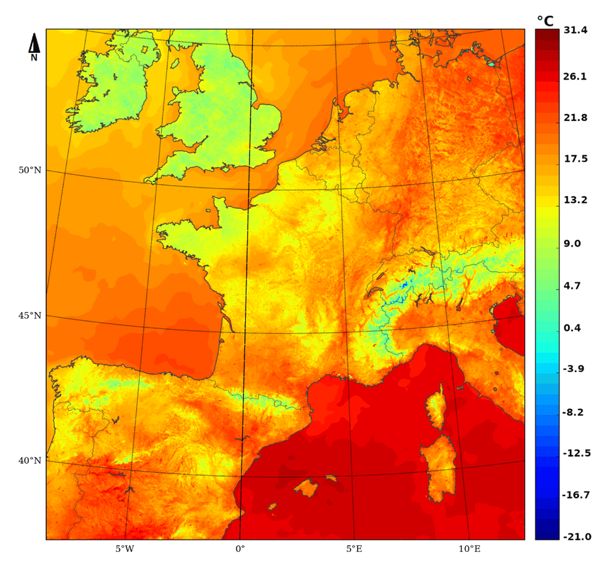
Figure 1
Geographical domain of AROME-France represented by Surface temperature field (°C) of September 1st 2019, 01 h range of 00 UTC forecast.
AROME is a spectral model derived from the global NWP model ARPEGE (Action de Recherche Petite Echelle Grande Echelle, (Courtier et al., 1991)). The current operational version (2020) used for this study has a 1.3 km × 1.3 km grid and 90 vertical levels from 5 m high up to 10 hPa. AROME is coupled to the ARPEGE global model and produces eight forecasts everyday at 00, 03, 06, 09, 12, 15, 18 and 21 UTC with a forecast range of 48 h for 00 and 12 UTC runs, of 45 h for the 03 UTC run, of 42 h for the 06 and 18 UTC runs and of 7 h for the 09, 15 and 21 UTC runs. AROME uses the dry thermal and shallow convection mass-flux convection scheme (Pergaud et al., 2009) and the TKE (Turbulent Kinetic Energy) turbulence scheme (Cuxart et al., 2000). In terms of radiation, the RRTM scheme (Mlawer et al., 1997) is used for long wave spectrum while the Fouquart-Morcrette scheme is used for the short wave spectrum. The land surface scheme uses SURFEX-ISBA-3L (Interaction Soil-Biosphere-Atmosphere) ((Noilhan and Planton, 1989) and (Boone et al., 1999)) with a surface initialization based on the force-restore method (2 layers for soil temperature and 3 layers for soil moisture content) with a dedicated analysis scheme (Giard and Bazile, 2000) described in the next section.
1.2 The 3D-var assimilation system in AROME-France model
AROME-France model uses a 3D variationnal assimilation scheme with 1 h assimilation window. The assimilated observations vary during the day but they consist in radiosondes, wind profilers, aircraft reports, ship and buoy reports, automated land surface stations, satellite observations, Global Positioning System Zenith Tropospheric Delay, and Doppler radar wind and humidity observations from radar reflectivities. Both satellite and conventional observations are assimilated in AROME upper air assimilation. Among these, radar observations represent the major part of assimilated conventional observations (around 75%) and represent around 60% of the total assimilated observations. Satellite observations represent around 20% of the total and are composed of wind observations from atmospheric motion vectors and scatterometers, microwave and infrared radiances. Infrared observations represent around 75% of satellite observations, with half of them coming from SEVIRI radiometer onboard Meteosat Second Generation, and the other half provided by IASI (Infrared Atmospheric Sounding Interferometer) hyperspectral instrument onboard Metop platforms.
The background used here is a 1h-forecast and background error statistics determine how an observation can modify analysed fields and how the information propagates from the observation location to other model points and to unobserved model variables. The background error statistics are estimated using forecast error statistics of vorticity, divergence, temperature, surface pressure and specific humidity. The background error covariance matrix is a climatological matrix, spatially homogeneous and isotropic, and is estimated using (Berre, 2000) multivariate formulation with an ensemble of differences of 3h range forecasts ((Brousseau et al., 2016)). The background error covariances were calculated from two periods of 15 days each of ensemble data assimilation with a limited number of members (6) at high resolution, one in summer and one in winter. It includes static covariances between variables and between different points of the 3D space for each variable. Recent developments within AROME model have proved the positive impact of a B matrix derived from ensemble data assimilation of the day, including covariances between variables and levels of the atmosphere and points of the space. This new B matrix results in a 3D-EnVar which improves forecasts of extreme events such as convective precipitation and winds. Concerning surface assimilation, some developments are ongoing to improve the optimal interpolation scheme and move towards a variational framework which could also benefit from the ensemble data assimilation. A 2D-EnVar is under development for AROME model surface assimilation with a B matrix derived from ensemble data assimilation of the day, including spatial covariances and covariances between variables, which could alleviate some of the optimal interpolation drawbacks which is univariate and has static background error statistics.
The variational analysis is performed every hour at the resolution of the model. The spin-up was reduced using a background error covariance matrix calculated from forecasts coming from an ensemble data assimilation at the AROME-France resolution, in order to simulate the evolutions of errors during the assimilation cycle (Brousseau et al., 2016). The increments obtained with these background errror statistics are more balanced and avoid the part of the spin-up coming from imbalanced analysis increments. Residual spin-up comes from imbalance between the model fields, and between the upper-air analysed fields and the surface fields that come from surface assimilation. It is noteworthy that the long-range (48 h) forecasts at 00 and 12 UTC also benefit from the analysis at 01 and 13 UTC, respectively, using an incremental analysis update (IAU) in order to improve their quality. It has been proven that the quality of forecasts updated using IAU is equivalent to the quality of forecasts initialized one hour later.
1.3 LST retrieval in AROME-France model
Satellite infrared and microwave instruments do not observe the Earth directly but measure the radiation reaching the top of the atmosphere. These radiations are the sum of the radiation emitted by the Earth surface, by the atmosphere and the radiation received and reemitted by the surface and the atmosphere. The approach of LST retrieval is based on the use of window channels for which the atmosphere is transparent in a way that the radiances observed by the satellite instruments result from the Earth surface emission only and are not impacted by the atmosphere in the absence of clouds. In order to calculate the surface parameters knowing the atmospheric state, the LST or surface emissivity retrieval needs to invert the radiative transfer equation ((Guedj et al., 2011) and (Karbou et al., 2006)):
where ∊v is the surface emissivity, Rv(θ) is the observed radiance, θv is the incidence angle, Γv is the atmospheric transmittance, Ts is the surface temperature, and are respectively the up-welling and the down-welling radiances for the channel ν. In case of surface temperature retrieval for infrared channels, the emissivity is taken from an emissivity atlas (Seemann, 2007) and the LST is given by the inverse form of the radiative transfer equation:
where L is the Planck function. Given the higher temporal and spatial variation of the surface temperature compared to 2 m temperature and the inaccurate representation of surface conditions in the model, previous studies (Karbou et al., 2006) and (Guedj et al., 2011) have shown the interest of using the retrieved surface parameters for the satellite radiances data assimilation. At Météo-France, the retrieval of surface temperature is performed for infrared instruments assimilation (SEVIRI and IASI) in clear sky. On the contrary, the retrieved surface emissivity is used to assimilate the microwave instruments knowing the larger variation of surface emissivity in the microwave bandwidth. The objective of the study is to assimilate the retrieved land surface temperature from SEVIRI in the land surface model of AROME model. (Sassi et al., 2019) have shown that the representation of the diurnal cycle with satellite derived land surface temperature is more accurate than the representation of the model, especially in spring and summer. It has also been shown in a previous study (Sassi et al., 2019) that the use of the land surface temperature retrieved from an instrument was useful for the simulation of the brightness temperature of other instruments and that it improves the simulations using the model surface temperature. These results were encouraging to develop the assimilation of satellite retrieved land surface temperatures in the surface scheme.
2 The surface model
2.1 SURFEX
SURFEX (Externalized surface) is a surface modelling platform developed at Météo-France (Masson et al., 2013) that can be used in offline mode or coupled to atmospheric models such as AROME. In coupled mode, the atmospheric model and SURFEX exchange atmospheric fluxes (radiation, precipitation) and near surface meteorological parameters (temperature, humidity, wind) from the atmosphere, and surface turbulent fluxes (heat, moisture, momentum) and surface temperature from the surface at each time step, as described in Figure 2. These surface quantities are computed over four different tiles representing the nature of the soil: nature (soil/vegetation), town (urban areas), lake and sea. Open water areas are assumed to be saturated surfaces with a temperature imposed from an external analysis. On the contrary, for the other tiles (nature and town), explicit surface energy and water balances are solved at each model time step. The Town Energy Balance (TEB) allows the estimation of various surface temperatures (roads, building walls and roofs) over urban areas. Details can be found in (Masson, 2000) but they are not useful for the current study which is focused on improving the soil temperatures of the nature tile. Here, the ISBA (Interactions Soil Biosphere Atmosphere) parametrization is used for the nature tile ((Noilhan and Planton, 1989) and (Noilhan and Mahfouf, 1996)) in its three-layer version (Boone et al., 1999). It predicts the evolution of two soil temperatures (a superfical one TG1 associated with the diurnal forcing τ1 (1 day) and a deeper one TG2 associated with longer time scales τ2 = 2πτ1 (about 6 days)) using the force-restore method first proposed by (Bhumralkar, 1975). It is important to point out that over snow-free surfaces, the surface temperature TG1 is representative of a mean value accounting for both bare soil and vegetation contributions in the nature tile (one single energy balance is solved). Such a mean value makes the comparison with satellite estimates rather straightforward, since the land surface temperature seen by a radiometer is a mixture of the longwave emission from various surface types present in the pixel. Regarding moisture reservoirs, in summer conditions (i.e. no soil water freezing), four prognostic variables are evolved with time : an interception reservoir Wr for the vegetation (rain, dew), a superficial soil reservoir Wg1 (that controls bare soil evaporation), a root-zone reservoir Wg2 (that controls plant transpiration), and a drainage reservoir Wg3 (that interacts with ground hydrology). For NWP, only the soil moisture reservoirs Wg1 and Wg2 are of importance in terms of initial contents (Mahfouf et al., 2009).
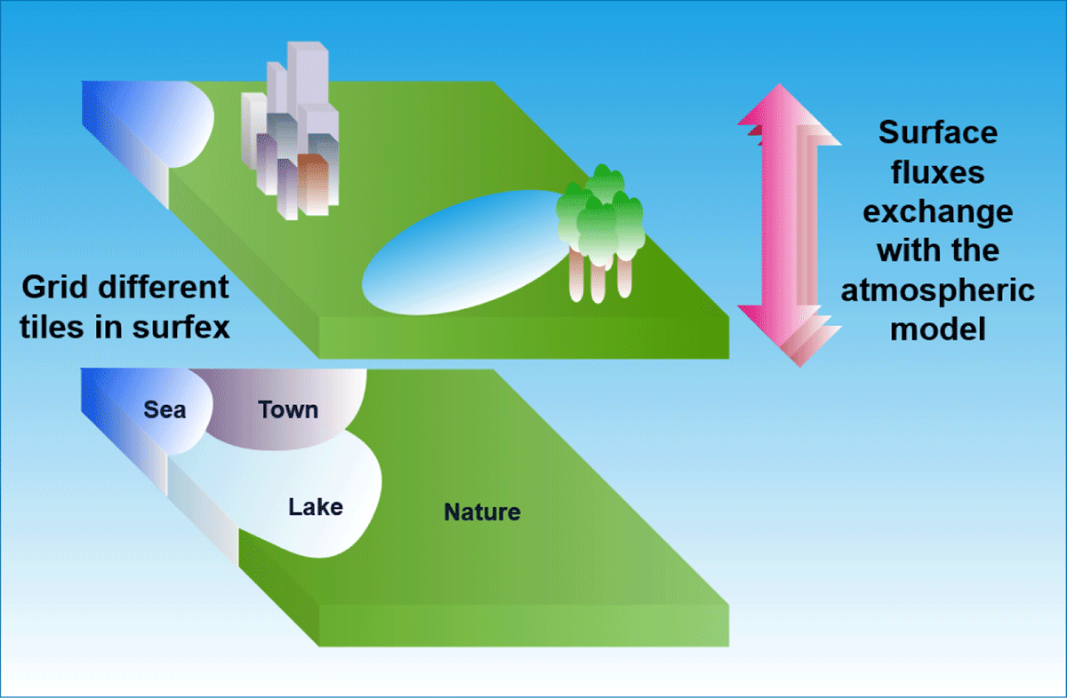
Figure 2
Description of SURFEX tiling and coupling with an atmospheric model.
2.2 The surface analysis system
A dedicated surface analysis scheme allows the initialisation of the soil prognostic variables of ISBA (Tg1, Tg2, Wg1, Wg2) every 3 hours even though the atmospheric analysis is performed every hour (this can be understood because deep soil variables evolve slowly in time with respect to atmospheric processes). This scheme that is described in (Giard and Bazile, 2000) is based on atmospheric increments of screen-level temperature (T2m) and relative humidity (RH2m), measured at two meters by synoptic (SYNOP) weather stations, in order to correct the four soil variables (Tg1, Tg2, Wg1 and Wg2). Therefore a first step is a bidimensional analysis of T2m and RH2m using surface weather stations (SYNOP reports and the French high density surface station network RADOME) and a short-range AROME forecast as background field. This is done by a univariate optimum interpolation scheme with mostly homogeneous and isotropic structure functions (some dependency with orography are accounted for as explained in (Soci et al., 2016)). The structure functions for T2m and Hu2m are as follows:
where dist is the distance between the observation and the analysis point and D is a characteristic distance, D is set to 100 km for T2m and Hu2m in AROME model. g(Δalti,ΔLSM) is the function accounting for differences between the land-sea mask of the observation and of the analysis point, and between the altitude of the observation and the analysis point. The T2m and Hu2m data benefit from an advanced quality control on observations. Observations with missing or wrong orography are rejected. Observations for which the difference between observation and the background is larger than for T2m for SYNOP and buoy observations, or larger than for Hu2m are rejected before the assimilation. Observations for which the innovation (obs-guess) is larger than for T2m or larger than for Hu2m are checked after analysis and they are kept if the analysis departure (obs-analysis) if lower than for T2m or for Hu2m (Stjepan, 2016).
In a second step, the T2m and RH2m analysis increments are used to correct the soil variables with linear relations. For soil moisture, optimal interpolation coefficients depending upon surface properties and atmospheric conditions as proposed by (Giard and Bazile, 2000) are used operationally. For soil temperature, these are empirical corrections initially proposed by (Coiffier, 1986) for a previous land surface scheme and adapted by (Giard and Bazile, 2000) to the ISBA scheme (Mahfouf et al., 2009), that is:
The atmospheric correction is imposed as such to the surface temperature Tg1 and is reduced for the deeper temperature Tg2 (to account implicitly for the heat wave damping). A similar scheme is also used at ECMWF for soil temperature (Douville et al., 2000) despite the use of a Simplified Extended Kalman Filter for soil moisture analysis (De Rosnay et al., 2013). The only difference with the Météo-France set-up is the use of an empirical function that prevents from correcting soil temperatures during daytime (since errors are more likely to arise from soil moisture from the turbulent fluxes). This operational methodology has been modified in order to include SEVIRI LST. First the bidimensional optimal interpolation has been adapted from T2m and RH2m observations to allow the bidimensional optimal interpolation of surface temperature with SEVIRI LST observations and the ISBA surface temperature Tg1 as a background field (1h forecast). The various parameters defining background and observation errors statistics (variances and correlation length) have been setup from the results of the diagnostic studies presented in Section 4. Then, the analysis increments ΔLST are used to modify the soil temperature increments as:
This first choice of equal weights between the two increments will have to be revised in the future when more optimal coefficients will be used for the soil temperature analysis. It allows to account for the LST information in the soil layers without discarding the information from screen-level variables. As explained later the use of SEVIRI LST in the soil analysis will be restricted to night time periods, in agreement with results from (Mahfouf, 2007) and the ECMWF set-up. When SEVIRI LSTs are not used, the soil temperature corrections are provided by equation 4. Figure 3 summarizes the implementation of SEVIRI LST assimilation in the surface analysis system together with the assimilation of screen-level data from surface observations.
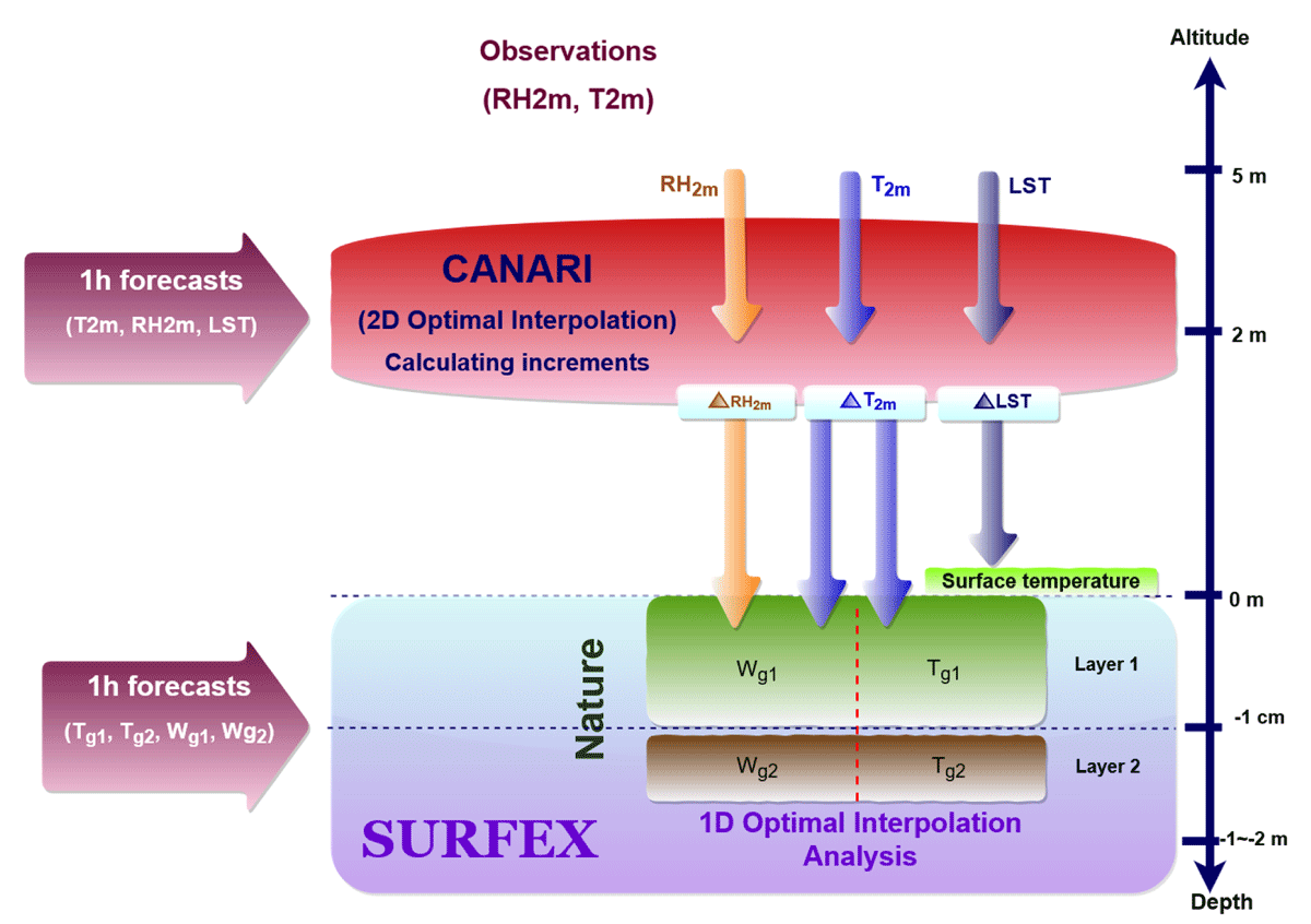
Figure 3
Implementation of the Land Surface Temperature assimilation in the surface analysis of AROME model.
3 Diagnostics of observation and background errors
The 2D optimal interpolation used for the surface analysis requires information about the observations and the model together with their associated errors. The observation error standard deviations are required together with the background error standard deviations. Moreover the horizontal correlation length is necessary to evaluate the horizontal correlations of temperature errors.
The spatial correlations of observation errors are indeed not taken into account in the OI framework which considers a diagonal R matrix. This limitation could possibly degrade the results of assimilating observations on a dense network such as SEVIRI observations. However, to alleviate this limitation, we applied a horizontal thinning in the assimilated observations so only one SEVIRI observation out of 5 has been considered in each direction, as it is done in the atmosphere for the 3D-Var analysis and we considered observation errors as not correlated.
The method used for the error diagnostics consists in a posteriori diagnostics as proposed by (Desroziers et al., 2005). This method is based on the background and analysis departures in order to estimate the error covariances. One iteration has been run to calculate the new error covariances which were close to the a priori ones. However, since the background error covariance precision is essential in the convergence of the diagnostics, several iterations can be processed in order to improve the definition of the statistics.
3.1 Diagnostics of observation errors
Using the Desroziers approach described in (Desroziers et al., 2005), the observation error covariances are diagnosed based on the analysis and the background departure statistics. The consistency check verifies the equation:
where R is the observation error covariance matrix, is the innovation vector, is the vector of differences between the observation and the analysis in the observation space and E is the mathematical expectation. The initial a priori values for the observation and background error standard deviation are 3 K and 1.5 K, respectively. As the diagnosed values are rather close to the arbitrary a priori values, only one iteration has been carried out (Bathmann, 2018). Following conclusions of (Sassi et al., 2019) that have shown that nighttime observations are closer to in-situ surface temperature observations than the model surface temperature, only nighttime observations have been considered here. Therefore only observations at 21, 00 and 03 UTC analysis times are first kept. However large observation standard deviations have been observed at 21 UTC, greater than 5 K over a large part of the domain, that is why the 21 UTC analysis time has been excluded form further experiments. The standard deviations over July and August 2019 of the observation errors for 00 and 03 UTC show spatial variability over the AROME-France domain as described in Figure 4 with smaller mean standard deviations over the southern part of the domain especially over the Iberian peninsula and higher values to the North especially over the United Kingdom.
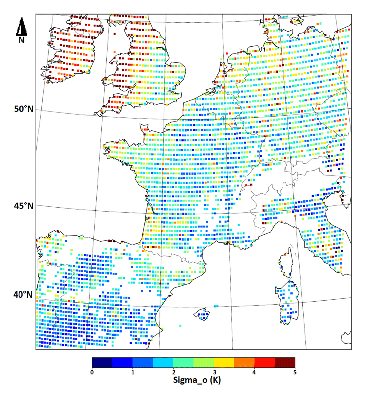
Figure 4
Standard deviations of diagnosed LST “observation” errors for July and August 2019 (00 and 03 UTC). The missing pixels are due to the application of an orography filter (see text for explanation).
The examination of the amount of observations used to calculate the standard deviation shows a consistent spatial variability of the number of available observations with the values of the diagnosed standard deviation. The higher standard deviations were observed in areas with a fewer number of clear observations, which might be due to a higher cloudiness. In fact, more observations are available over the southern part of the domain (around 100 clear observations per pixel) than over the norther part (around 50 clear observations per pixel), and larger standard deviations in average are observed over the northern part of the domain. Standard deviations of observation errors vary from 1.5 K to 4.5 K at some places.
Over the major part of the domain the standard deviation is between 1.5 and 2.5 K. Slightly larger observation errors up to 3 K are observed over some parts of the Iberian peninsula, which can be related to semi-arid regions. Larger values over 3 K and up to 4.5 K are observed over the northern part of the domain, which can be related to regions with a smaller amount of pixels entering the analysis. These regions are also characterized by wet soils and possible undetected or misclassified clouds impacting the diagnostics, which should be done only for clear sky.
Hereafter we have applied an orography filter that rejects observations over high or complex orography. In fact, pixels with altitude higher than 1000 m and those for which the standard deviation of altitude points with surrounding pixels (in a 10 km radius) is above 100 m have been discarded in the computation of the error statistics. This double filter enabled rejecting the observations above orographic areas and also the areas with high orographic gradients while keeping observations on mid-altitude plateaux. The rejected observations are located mainly over the Alps, the Pyrenees, the Massif Central, the Iberic Monts, the Guadarrama mounts and the Cantabriques mounts (as shown in Figure 4).
3.2 Diagnostics of background errors
In addition to observation error covariances, we have diagnosed the background error covariances using a similar approach based on the Desroziers method (Desroziers et al., 2005).
where B is the model error covariance matrix, H is the tangent linear version of the observation operator and HT its adjoint version, is the vector of differences between guess and analysis, and is the innovation vector.
Figure 5 shows the mean background error standard deviations for 00 h and 03 h analysis times of July and August 2019. Background errors appear to be more homogeneous compared to the observation ones as displayed in figure 4. We also notice smaller standard deviation in average for the background errors compared to the observation errors with maximum values around 1 K in most cases. However, these values exceed 1.5 K over few locations such as near mountainous areas for example over the Iberian peninsula. This fact might be explained by a misrepresentation of sub-grid heterogeneities. According to these diagnostics, we considered as tunings for the following part an observation error of 3 K and a background error of 1.8 K for the SEVIRI LST assimilation. Note that the observation and background errors for the 2 m temperature are respectively of 1.4 and 1.6 K as in the operational version of AROME. Moreover, diagnostics of spatial error correlations have been carried out on the background surface temperature (not shown). They show that from 10 km the correlation between two points is reduced by 50% and from 30 km background error correlation is close to zero and the points can be considered as uncorrelated. Therefore we chose a correlation length of 30 km for LST error. In comparison the correlation length of 2 m temperature error is 100 km in the operational version of AROME and is kept to the same value in the following experiments.
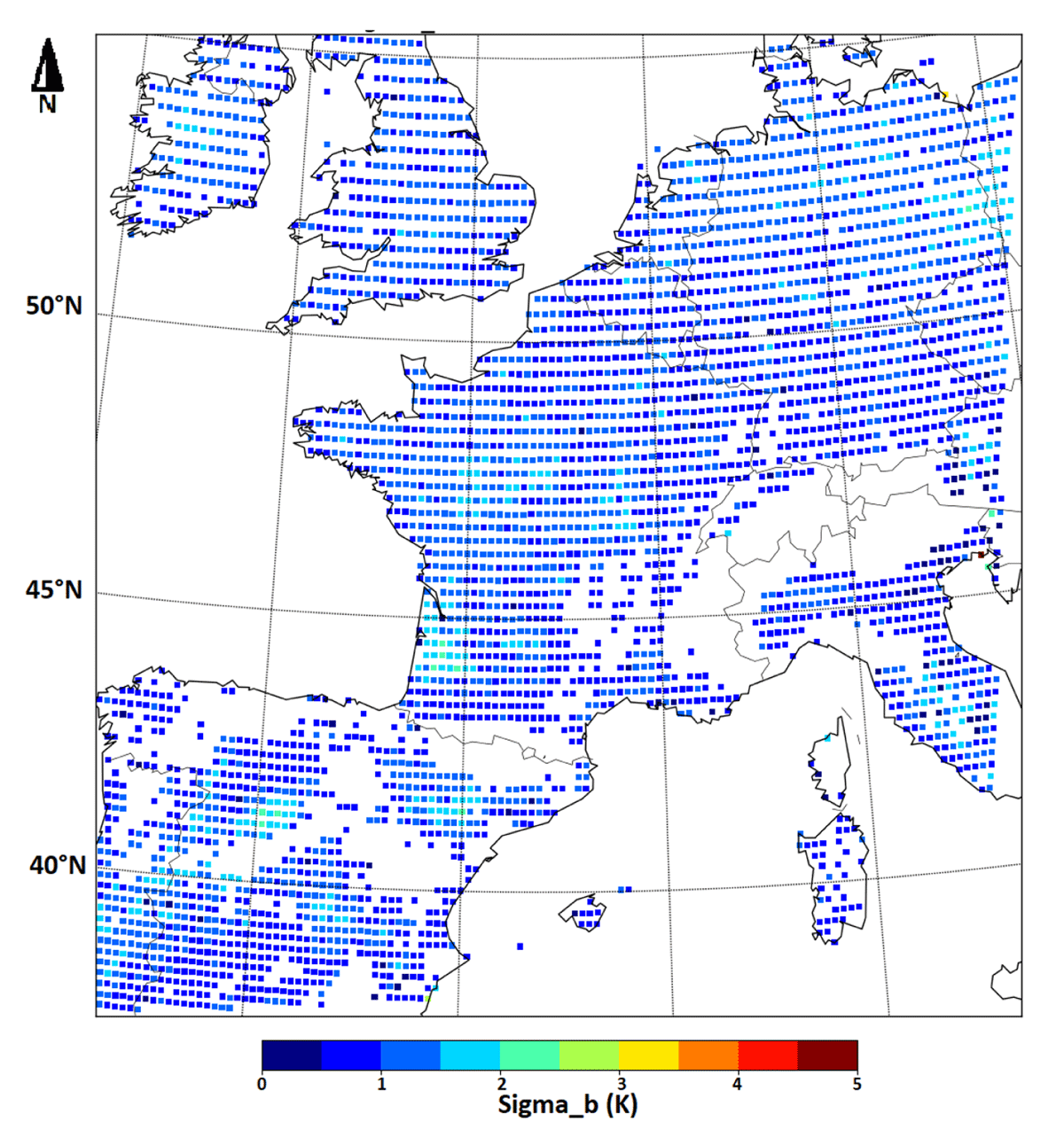
Figure 5
Standard deviations of LST model errors for July and August 2019 (00 and 03 UTC).
4 Experimental design and results
4.1 A case study: La Loire basin sub-domain
For a first experimental set-up, we chose a summer period covering July and August 2019 to assimilate clear sky SEVIRI LST to optimize the number of clear sky data. We rely on the NWC SAF (Le Gleau, 2019) cloud classification provided with the SEVIRI data to select pixels classified as “clear over land”. A spatial thinning is also applied with one pixel retained out of five. This corresponds to the operational thinning ratio used in the atmospheric analysis. Finally only nighttime pixels are assimilated since the observation error standard deviations are rather low by nighttime, as demonstrated in the previous section, and as previous studies showed that LSTs retrieved from different infrared sensors agree better during nighttime (Sassi et al., 2019). In order to understand the impact of the SEVIRI LST assimilation, we considered a sub-domain within the AROME-France domain and located in the North-Western part of France, near the Loire river estuary (3 W – 0.5 E, 46,5N 48,5 N).
Figure 6 shows the surface temperature from the 1h forecast in addition to SEVIRI retrieved LST (squares) and 2 m temperature (circles) for July, 4th 2019 at 03 UTC on the Loire basin sub-domain. The south-western part of the domain (surface temperature varying between 291 and 292 K) corresponds to the Atlantic Ocean. Figure 6 shows a high spatial variation of surface temperature in the background from the North to the South, with up to 5 degrees difference. Moreover, we notice a global qualitative agreement between the model surface temperature, the SEVIRI LSTs and the 2 m temperatures. However, few SEVIRI LSTs show higher differences (colder by more than 4 K) with model surface temperature and other neighboring SEVIRI LST and 2 m temperature observations. To help understanding these differences, we show in Figure 7 the surface temperature differences between analysis and guess while assimilating SEVIRI LST only (no 2 m temperature observations have been assimilated at this stage).
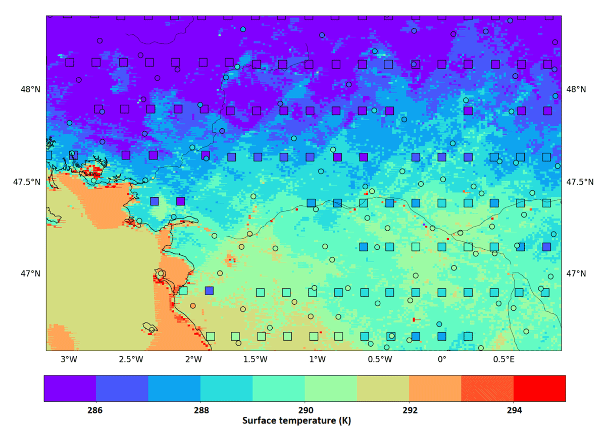
Figure 6
Model surface temperature from 1-h forecast (K, colors), T2m observations (K, circles) and SEVIRI Land Surface Temperature (K, squares) for the July 4th 2019 at 03 UTC over the Loire river basin sub-domain.
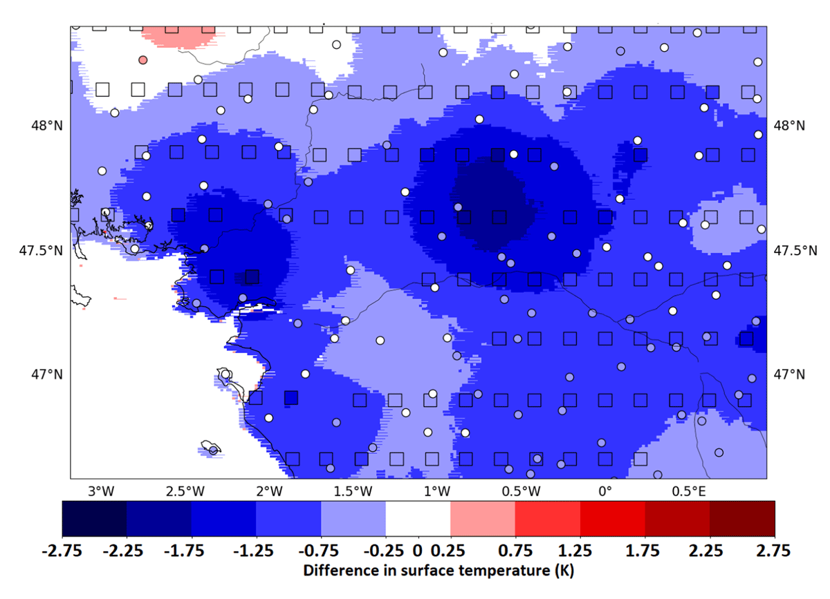
Figure 7
Differences in surface temperature (K) between guess and analysis (colored areas) and increments of analysis at SEVIRI pixel locations (K, squares) and at T2m observation locations (K, circles) for the July 4th 2019 at 03 UTC on the “La Loire” basin sub-domain.
Two large negative areas of LST analysis increments can be noticed at 47.75 N, 0.5 W and 47.4 N, 2 W. After having performed 2D OI SEVIRI using LST and 2m temperature analysis, surface temperature analysis increments can be derived as shown in Figure 8. The use of 2m temperature analysis, warmer than SEVIRI LST by more than 2 K over the two negative areas has reduced the amplitude of these increments.
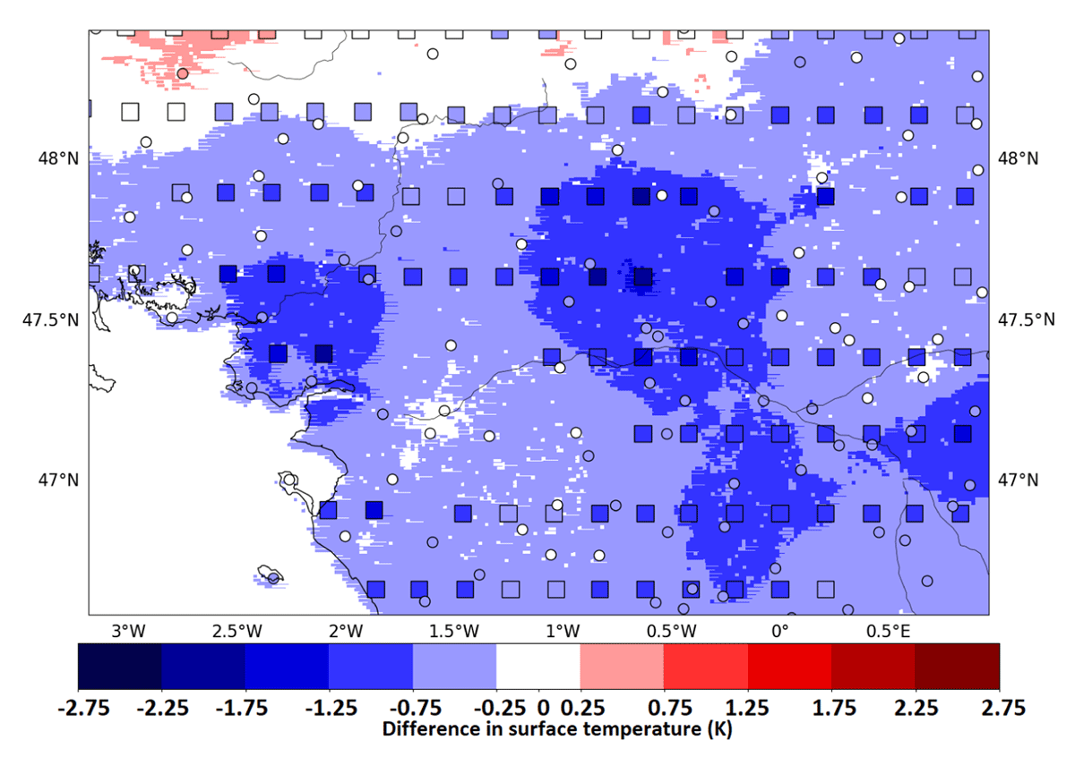
Figure 8
Analysis increments (difference between observations – analysis) of the first soil layer temperature (K) after the surface analysis using the SEVIRI LST and the T2m observation (colors) and increments of analysis on SEVIRI pixels (K, squares) and on T2m observation locations (K, circles) for the July 4th 2019 at 03 UTC over the Loire river basin sub-domain.
From this example, the SEVIRI LSTs show high variability at small spatial scales. One possible reason might be the presence of clouds misclassified as clear sky pixels that could induce the observed cold bias. To further investigate this hypothesis, we evaluated the first guess departures distribution for the SEVIRI LST for July and August 2019 at 03 UTC as shown in Figure 9.
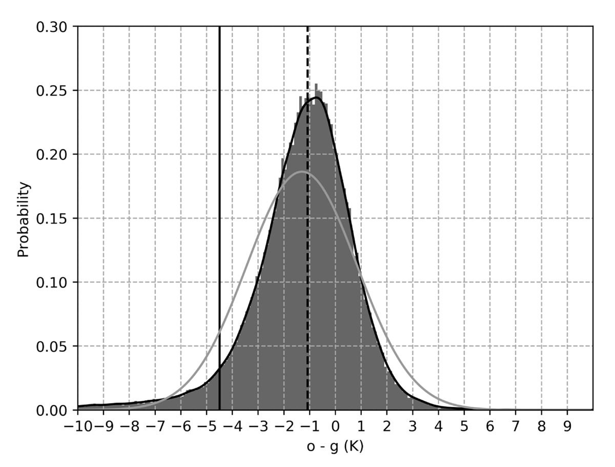
Figure 9
Background departures (obs – guess) distribution for all the 03 UTC analysis time of July and August 2019 with the best fit distribution in black line and normal distribution in gray line. The vertical dashed line indicates the median whereas the continuous line indicates the -4.5 K threshold.
We notice a cold residue that might be due to a mismatch in cloud type detection. In order to reduce such impact on the assimilation, we considered, as an additional criteria, a background departure threshold of –4.5 K below which the LST is rejected from the analysis.
After evaluating the impact of SEVIRI LST on surface temperature analysis, and in order to assess its impact on atmospheric parameters, we have performed a two month experiment (EXP-ARO) in which we consider SEVIRI LST assimilation at 00 and 03 UTC on top of 2 m temperature and relative humidity already assimilated every three hours in the operational version of AROME model surface analysis. We took then into account the findings of the previous work to improve the experimental set-up. While the observation and background errors of 2 m temperature remain equivalent to the operational version, we maintained the observation and background errors of LST, previously defined for the case studies, at respectively 3 and 1.8 K and also the correlation length of LST errors at 30 km. Table 1 summarizes the main settings of the assimilation experiment (EXP-ARO) and also the control experiment (REF-ARO) that reproduces the operational AROME configuration. We present in the following sections the impact of SEVIRI LST assimilation, first on the assimilation of different parameters and then on AROME forecasts.
Table 1
Setups of the reference and the SEVIRI LST assimilation experiments.
| REFERENCE1 | EXPERIMENT | |
|---|---|---|
| REF-ARO | EXP-ARO | |
| Assimilation of T2m | Yes (00, 3, 6, 9, 12, 15, 18, 21) | Yes (00, 3, 6, 9, 12, 15, 18, 21) |
| Assimilation of LST | No | Yes (00 and 03 UTC) |
| Experiment period | from 05/07/2019 to 04/09/2019 | from 05/07/2019 to 04/09/2019 |
| Horizontal correlation length (T2m) | 100 km | 100 km |
| Standard deviation of observation error (T2m) | 1.4 K | 1.4 K |
| Standard deviation of background error (T2m) | 1.6 K | 1.6 K |
| Horizontal correlation length (LST) | – | 30 km |
| Standard deviation of observation error (LST) | – | 3.0 K |
| Standard deviation of background error (LST) | – | 1.8 K |
4.2 Impact on assimilation
The first step to evaluate the SEVIRI LST assimilation in the AROME model was to evaluate its impact on surface and atmospheric analyses in terms of improvement of model guess compared to observations. For temperature, we evaluated the statistics of innovations (observation – guess) at 2 m compared to surface stations observations (synoptic stations). Figure 10 shows the mean differences between the 2 m temperature observations and the model short range (1 h) forecasts as a function of the analysis time for EXP-ARO and REF-ARO experiments.
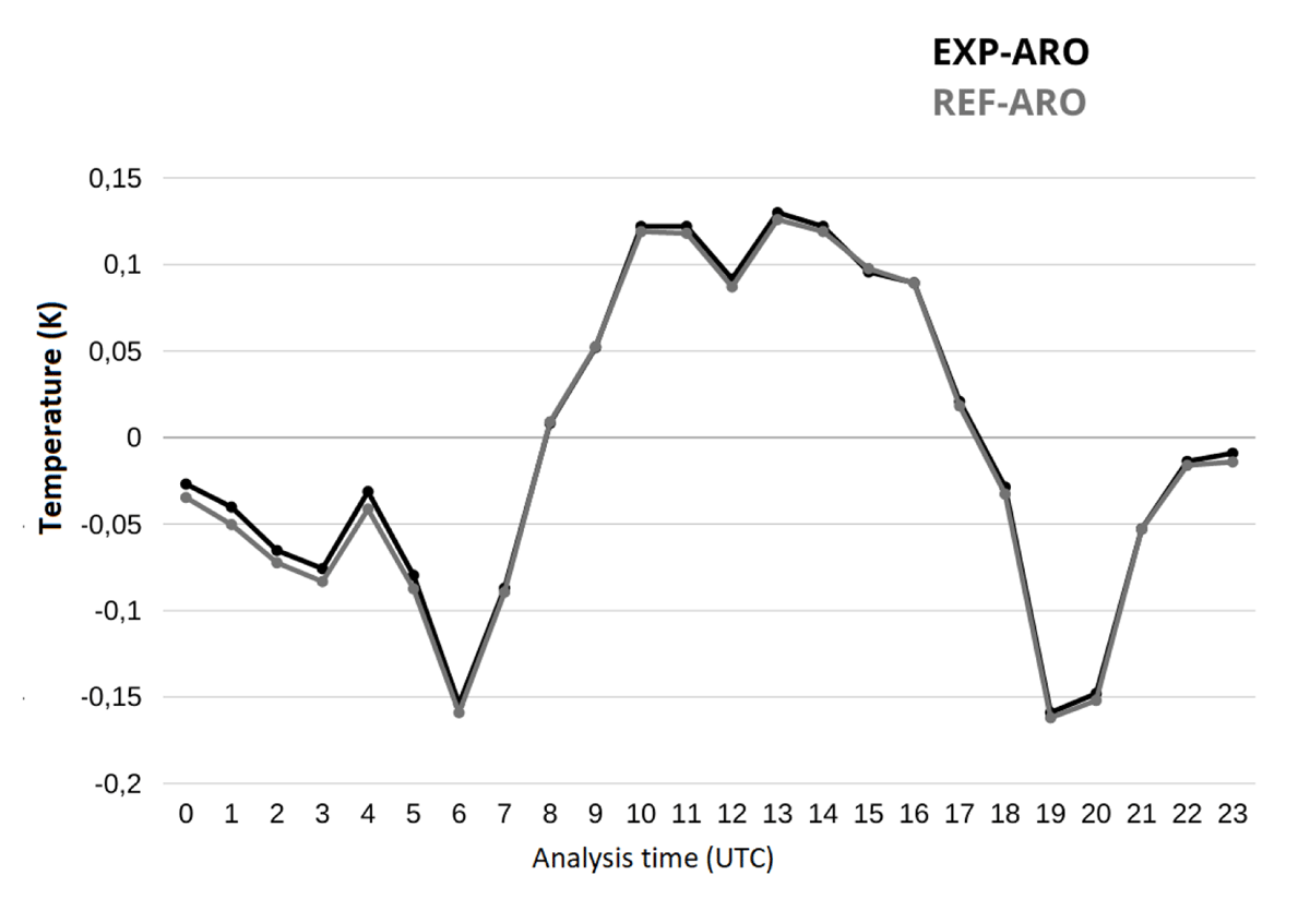
Figure 10
Mean differences over July and August 2019 between 2~m temperature (K) observations and background for EXP-ARO (black line) and REF-ARO (grey line) experiments for each analysis time.
Figure 10 shows, during night-time (up to 6 UTC), a slight decrease in the 2 m temperature mean innovation difference for EXP-ARO compared to REF-ARO, which represents an improvement of the background quality as it is closer to independent observations. This is consistent with the fact that SEVIRI LST have been used only at 00 and 03 UTC. Moreover, we notice a slight decrease in the mean differences on the last assimilation times of the day (19 UTC – 00 UTC). This might be due to a better short range forecast closer to the observation, due to better surface temperature in the forecast. This improvement indicates that the assimilation of SEVIRI LST has still an impact 15 to 21 hours later the assimilation time (at 00 and 03 UTC). However, a slight increase in the mean differences for EXP-ARO with respect to REF-ARO are noticed around noon (10 UTC – 14 UTC) despite the fact that no SEVIRI LST are assimilated during the day.
In addition to 2 m temperature innovations, we compared the mean differences between 2 m relative humidity observation and model background for EXP-ARO and REF-ARO as described in Figure 11.
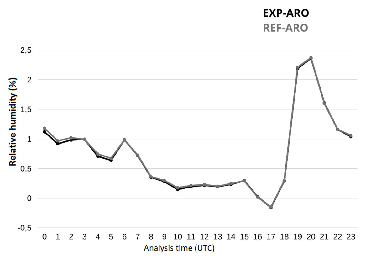
Figure 11
Mean differences over July and August 2019 between 2~m relative humidity (%) observations and background for EXP-ARO and REF-ARO for each analysis time.
Consistently with what has been noticed for the 2 m temperature, the mean differences slightly decrease with EXP-ARO compared to REF-ARO not only during the first assimilation times but also around noon and at the end of the day. However, the impact is very small after 6 h.
Furthermore, in order to evaluate the impact of SEVIRI LST assimilation on the assimilation of satellite observations, we considered microwave instruments in the atmospheric component of the model, since the model surface temperature is used to retrieve surface emissivity in a window channel for each microwave instrument in order to assimilate the other channels. Consequently, a modification of the model surface temperature is expected to induce an impact on the model equivalent to observations and then on the assimilation of microwave channels. For infrared sensors, as mentioned before, a LST is retrieved separately for each sensor to assimilate its sounding channels. We present in Figure 12 the impact of the SEVIRI LST assimilation on MHS microwave sensor which has shown the most significant impact, especially for the channel 5 (183 GHz+/– 7) sensitive to water vapour absorption at 700 hPa in terms of RMSE (Root Mean Square Error) differences in %.
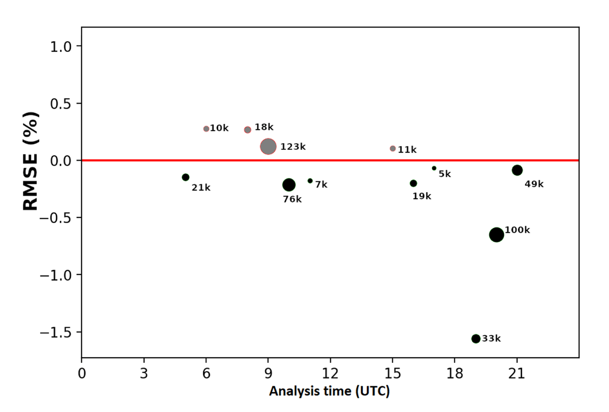
Figure 12
Relative difference between MHS channel 5 observed and 1 h forecast radiances for July and August 2019. The negative values correspond to an improvement of the channel 5 simulation with EXP-ARO compared to REF-ARO. The size of the symbols indicate the number of assimilated observations.
We notice an improvement in MHS channel 5 assimilation with EXP-ARO over most of analyses times (corresponding to negative values of relative RMSE differences), and not only around 0 and 3 UTC at which SEVIRI LST are assimilated. This could result from a more realistic surface temperature obtained in EXP-ARO compared to REF-ARO which propagates in time. It might be interesting to evaluate the impact of the assimilation of LST at all analysis times, also during daytime with adequate observation error statistics, in order to investigate if a larger improvement is obtained in the microwave radiances assimilation.
4.3 Impact on forecasts
A first evaluation of the SEVIRI LST assimilation on the forecast quality has been considered according to surface parameters using surface stations (synoptic + RADOME) observations represented in Figure 13. The number of observation remains the same all along the day.
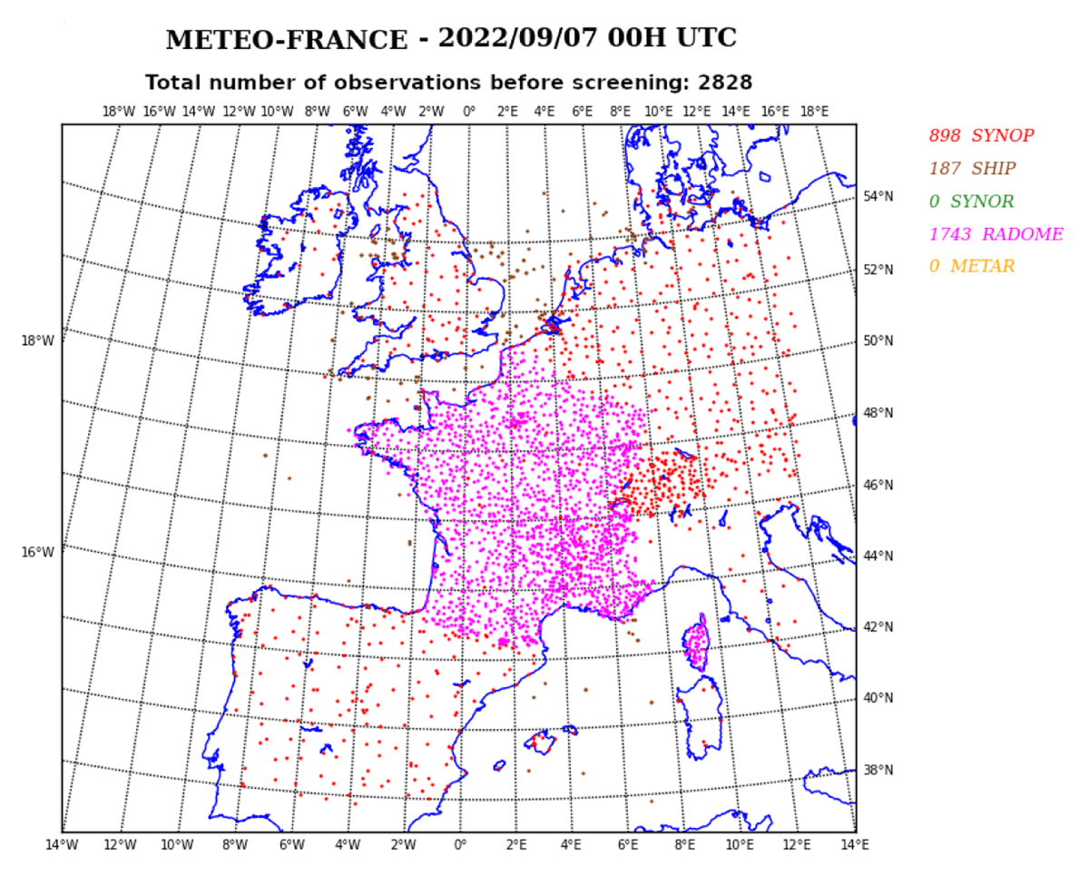
Figure 13
Map of coverage of surface observations available on September 7th 2022 and used in AROME-France model.
Various meteorological parameters have been evaluated, and we focus here on 2 m temperature and relative humidity, that show small but significant impacts especially by nighttime. Table 2 gives the differences of RMSE for the 2 m temperature and relative humidity parameters according to forecast range. Positive values indicate an improvement of EXP-ARO with respect to REF-ARO.
Table 2
Differences in RMSE of 2 m temperature (K) and 2 m relative humidity (%) forecast (ranges between 0 to 48 h) between REF-ARO and EXP-ARO compared to surface stations observations for July and August 2019. Positive values correspond to an improvement with EXP-ARO. Bold values represent the significant impacts according to Bootstrap test with a minimum of 95% confidence level.
| 0 H | 6 H | 12 H | 18 H | 24 H | 30 H | 36 H | 42 H | 48 H | |
|---|---|---|---|---|---|---|---|---|---|
| 2 m Temperature (K) | –0.01 | 0 | 0 | 0 | 0.01 | 0.01 | 0 | 0.01 | 0.01 |
| 2 m Humidity (%) | –0.02 | 0.01 | 0.04 | 0.08 | 0.06 | 0.06 | –0.02 | 0.01 | 0.07 |
Table 2 shows small but significant impacts at different forecast ranges. First, for 2 m temperature, a very small increase in RMSE at the analysis time 0 UTC with EXP-ARO is noticed. This fact can be explained by the assimilation of SEVIRI LST that increases the distance between the analysis of EXP-ARO and the 2 m temperature observations, compared to REF-ARO that assimilates only 2 m temperature for the soil temperature analysis. On the other hand, there is a slight and significant improvement in 2 m temperature forecast at nighttime forecast ranges (24 h and 48 h). This behaviour can be explained by a better analysis of surface temperature thanks to the SEVIRI LST assimilation leading to more realistic surface temperature forecasts.
For 2 m relative humidity, significant positive impacts take place during nighttime forecast ranges (18 h to 30 h and 48 h). These improvements of the nighttime forecast range have also been found for the 2 m temperature parameter. This shows that SEVIRI LST assimilation at 00 UTC and 03 UTC assimilation times has given a consistent impact on the nighttime forecasts for both temperature and relative humidity parameters at 2 m.
To further assess the impact of SEVIRI LST assimilation, temperature and relative humidity forecasts in the atmosphere are evaluated at various heights using radiosonde observations at 1000, 850, 700, 500 and 400 hPa (Table 3).
Table 3
Difference in RMSE of temperature (K) and relative humidity (%) forecasts (ranges up to 48 h) between REF-ARO and EXP-ARO compared to radiosonde observations at 1000, 850, 700, 500 and 400 hPa. Positive values correspond to an improvement with EXP-ARO with respect to REF-ARO. Bold values represent significant impacts according to Bootstrap test with a 95% confidence level.
| 0 H | 12 H | 24 H | 36 H | 48 H | ||||||
|---|---|---|---|---|---|---|---|---|---|---|
| T (K) | RH (%) | T (K) | RH (%) | T (K) | RH (%) | T (K) | RH (%) | T (K) | RH (%) | |
| 400 hPa | 0.01 | 0.02 | 0.01 | 0.7 | –0.01 | 0.07 | 0 | 0.01 | 0 | 0.07 |
| 500 hPa | –0.01 | 0.18 | 0 | –0.19 | 0.01 | –0.02 | 0 | 0.24 | 0 | –0.21 |
| 700 hPa | 0.01 | 0.4 | –0.01 | –0.71 | –0.02 | 0.03 | –0.01 | –0.31 | 0 | –0.04 |
| 850 hPa | 0 | 0.07 | 0 | 0.22 | 0 | –0.15 | 0 | 0.04 | 0.02 | 0.05 |
| 1000 hPa | 0.03 | 0.02 | 0.03 | –0.01 | 0.02 | –0.04 | –0.03 | –0.17 | –0.03 | 0.06 |
In terms of temperature, Table 3 shows small but significant impact of SEVIRI LST assimilation on the forecast up to 700 hPa level with a maximum amplitude of 0.03 K at 1000 hPa level. The significant impacts on forecast quality with EXP-ARO remain for the first 24 h range. After 24 h, the impact turns to be neutral to slightly negative.
In terms of relative humidity, Table 3 shows an improvement in forecast at 0 UTC that is maximum between 850 and 500 hPa, reaching 4 % of RMSE difference at 700 hPa, which is consistent with the Figure 12 showing smaller RMSE for water absorption channel 5 (sensitive to 700 hPa). For forecast ranges from 12 h to 48 h, significant impacts are mainly observed at 850 and 700 hPa with positive impact at 850 hPa at 12, 36 and 48 h, and a slight degradation at 24 h and at 1000 hPa at 12, 24 and 36 h with a maximum amplitude around 0.7% on both sides. These results are consistent with the temperature forecast evaluation. The consideration of these two parameters for verification is based on the operational verification system available at Météo-France which considers relative humidity close to the surface which is indeed correlated to temperature.
The above results have shown small but significant impacts mainly on surface and low levels temperature and relative humidity forecasts. We remind that during this experiment, as it represents the first LST assimilation work with the AROME model, we have chosen to assimilate the nighttime SEVIRI LST only and also to consider equal assimilation weights for SEVIRI LST and 2 m temperature for soil analysis. The different results will be summarized and these hypothesis will be further discussed in the next section.
5 Discussions and conclusions
This study represents the first work in AROME model in which the LST assimilation has been implemented in the surface analysis system. As a first step, the SEVIRI LST has been projected onto the model grid using a bidimensional univariate optimal interpolation scheme in a similar way as 2 meter temperature and relative humidity observations from surface weather stations. Secondly, the SEVIRI LST analysis increments have been used in addition to the 2 m temperature increments for the temperature analysis of the first two soil layers. At this stage, we considered equal weights between the LST and T2m increments during the soil analysis. Furthermore, we decided to consider the SEVIRI LST assimilation in AROME model at nighttimes only based on previous study assimilating LST by night (Candy et al., 2017) and previous work (Sassi et al., 2019). This previous work evaluated the synergy between different infrared and microwave sensors derived LST showing better synergy during nighttime and summer period. We also considered model and observation error diagnostics that showed smaller error standard deviations during nighttime.
The evaluation of the impact of the LST assimilation on the assimilation of other parameters has been conducted first using screen level observations. The assimilation of SEVIRI LST in AROME model over a period of two months covering July and August 2019 showed smaller departures of 2 meter temperature with a RMSE decrease of 0.01 K and relative humidity with a first-guess RMSE decrease of around 0.07% during nighttime. Moreover, the MHS microwave channel 5 simulation which is sensitive to humidity in the lower layers of the atmosphere showed reduced RMSE values at most of assimilation times up to 1.5%.
In addition to impact on the observation assimilation, we also considered radiosonde observations to evaluate the impact of LST assimilation on the forecast quality of temperature and humidity fields. On one hand, the assimilation of LST reduced the RMSE of temperature forecasts up to 700 hPa by up to 0.03 K. On the other hand, a consistent improvement of relative humidity forecast has been noticed in most cases mainly between 850 and 500 hPa with a maximum RMSE reduction of 4% compared to observations.
The evaluation of SEVIRI LST assimilation impact in AROME showed in most cases satisfying results and encourage to consider the evaluation of satellite derived LSTs at a larger scale. Yet, several improvements should be considered. The different aspects and weaker points of the study to be addressed in future studies concern the LST retrieval, the frequency of LST assimilation, the methodology to propagate LST increments into the soil and the soil variables impacted, and future work towards coupled soil-atmosphere assimilations.
On one hand, at the level of LST data itself, the retrieval methodology from infrared instruments using a fixed emissivity can be improved. We have considered during this work an LST retrieved from SEVIRI only using the operational mono channel retrieval method and a surface emissivity atlas as used in operations. However, we note that the emissivity atlas used for SEVIRI LST retrieval is different from the emissivity atlas used for other infrared sensors. In this direction, it would be worth to investigate the impact of SEVIRI LST assimilation while using a common emissivity atlas for all infrared sensors. To go further towards infrared sensor synergy, we can investigate the use of a different retrieval method that allows a simultaneous retrieval of LST and surface emissivity over land. It would be interesting also to evaluate the benefit of assimilating LST retrieved from different sensors in the infrared, together with surface information on surface temperature or moisture provided by channels in the microwave bandwidths.
On the other hand, the frequency of LST assimilation and the analysis times at which it is assimilated can be more in depth studied and improved. We have been focusing during this work on the LST assimilation impact during nighttime only, during which a better LST synergy has been previously observed and smaller error standard deviations have been found for both model and LST observations. The evaluation of LST assimilation impact on observations assimilation and forecasts showed most of improvement during nighttime. This encourages us to extend this study to cover more assimilation times based on zenithal angle variation over the AROME domain or further to extend the LST assimilation to daytime analysis times and also over different periods of the year. An adequate representation of model and observation errors during these new periods and analysis times is then mandatory, since we have found higher error standard deviations during daytime for model and especially for LST observations. This requires new diagnostics of model and observation error standard deviations allowing to attribute adequate errors to each. It would be also interesting to evaluate the impact of SEVIRI assimilation on hourly analysis basis instead of the three hourly current operational surface analysis.
Furthermore, the retrieved LST can be informative for different soil variables. As a first LST assimilation study in AROME, we have considered the LST increments in the analysis of soil temperature only. However, the 2 meter temperature is indeed used in complement of the 2 m relative humidity for the initialization of the soil moisture. The sensitivity of soil water content in the different soil layers to the LST shall then be evaluated for the soil moisture analysis. At a further step, it would be interesting to evaluate the impact of microwave observations assimilation in the soil moisture analysis.
Finally, the methodology used to propagate LST increments in the soil for soil temperature can be improved by accounting for more realistic sensitivities. Knowing the high coverage of surface observations over AROME-France domain, we have considered as a first study an equivalent weight of LST and 2 m temperature to analyze the soil temperature in the first and second layers. This choice can be improved by considering their respective observation errors in soil temperature analysis and the sensitivity of the temperature in each layer of the soil to LST and 2 m temperature. A more realistic consideration of error covariances will enable to better take into account the vegetation components. We remind that we observed higher model and observation error standard deviations in forest areas. This approach will improve the LST assimilation on different geographical domains which have wide tall and dense vegetation or also sparse coverage of 2 m temperature observation and will allow as a first step the LST assimilation in a global model such as ARPEGE for which the spatial distribution of surface observation is very heterogeneous.
This work constitutes the first effort towards a coupled assimilation system at Météo-France, by improving the consistency between surface and atmospheric assimilation regarding surface temperature over land surfaces. Further steps will involve the use of background information provided by ensemble of data assimilation for surface parameters. In this framework the assimilation of LST is crucial as an observation which provides information at the interface between surface and atmosphere.
Abbreviations
The following abbreviations are used in this article:
| LST | Land Surface Temperature |
| OI | Optimal Interpolation |
| SURFEX | SURFace EXternalisée |
| T2m | 2 meters temperature |
| RH2m | 2 meters relative humidity |
| NWP | Numerical Weather Prediction |
| UTC | Universal Time Coordinated |
| MSG | Meteosat Second Generation |
| IASI | Infrared Atmospheric Sounding Interferometer |
| SEVIRI | Spinning Enhanced Visible and Infrared Imager |
| AROME | Applications de la Recherche à l’Opérationnel à Méso-Echelle |
| CNRM | Centre National de Recherches Météorologiques |
| MW | Microwave |
| IR | Infrared |
| RTTOV | Radiative Transfer for TOVS |
| TOVS | TIROS Operational Vertical Sounder |
Funding information
The PhD of Mohamed Zied Sassi was funded by Météo-France and Région Occitanie. This research has been partly funded by CNES in the frame of IASI APR.
Competing Interests
The authors have no competing interests to declare.
Author contributions
Conceptualization, N.F., V.G., C.B.; methodology, N.F., V.G., C.B. and Z.S.; software, N.F., V.G., C.B. and Z.S.; validation, N.F., V.G., C.B. and Z.S.; formal analysis, N.F., V.G., C.B. and Z.S.; investigation, N.F., V.G., C.B. and Z.S.; resources, N.F., V.G., C.B. and Z.S.; data curation, N.F., V.G., C.B. and Z.S.; writing—original draft preparation, Z.S.; writing—review and editing, N.F., V.G. and C.B.; visualization, Z.S.; supervision, N.F., V.G., C.B.; project administration, N.F. and V.G.; funding acquisition, N.F.