
1. Introduction
Due to climate warming, many studies have shown the increasing trend of recurrent occurrences of drought hazards in several parts of the world (Sharma and Goyal, 2020; Shao and Kam, 2020; Liang et al. 2018; Nam et al. 2015; Kousari et al. 2014; Damberg and AghaKouchak, 2014; Gocic and Trajkovic, 2013). Many consequential studies, statistical facts, and figures have revealed the significant damages of drought in various discipline of life (Andriano and Behrman, 2020; Carroll et al. 2009). On the same lines, many studies have reported the continuation of drought in many parts of the globe. Drought directly affects human lives (Yao et al. 2018), agriculture crop yield, livestock (Nembilwi et al. 2021), and ecosystem (Haile et al. 2019). In addition, drought creates several issues related to public health such as poor sanitation and low quality of drinking water (Mullin et al. 2020). However, the adverse impact of drought can be reduced by proper planning and appropriate drought mitigation policies.
In contrast to other natural hazard, drought is complex and difficult to assess accurately as well as efficiently. Therefore, accurate drought monitoring and forecasting are necessary for early warning drought mitigation polices. For drought monitoring and forecasting, many authors have proposed and recommended several drought monitoring tools and forecasting methods. Some popular and new drought monitoring tools are, Palmer Drought Severity Index (PDSI) (Palmer, 1965), Standardized Precipitation Index (SPI) (McKee et al. 1993), Standardized Precipitation Evapotranspiration Index (SPEI) (Vicente et al. 2010), Joint Deficit Index (JDI) (Kao et al. 2010), Multivariate Standardized Drought Index (MSDI) (Hao et al. 2013), Multivariate Standardized Precipitation Index (MSPI) (Bazrafshan et al. 2014), Composite Drought Index (CDI) (Liu et al. 2020), Seasonally Combinative Regional Drought Indicator (SCRDI) (Ali et al. 2020), Regional Multi-Component Gaussian Hydrological Drought Assessment (RMcGHDA) (Ali et al. 2021), etc. Similarly, many researchers have developed several forecasting and prediction methods using various time series and machine learning approaches. For instance, Aghelpour et al. (2020) forecasted Joint Deficit Index (JDI) and MSPI under machine learning methods and entropy theory. Khan et al. (2020) utilized the strength of wavelet transformation and has proposed a hybrid model of Autoregressive Integrated Moving Average Model (ARIMA) and Artificial neural network (ANN) for drought predication. Pham et al. (2021) have forecasted drought based on SPI using Singular Spectrum Analysis (SSA) and Single Least Square Support Vector Machine (LSSVM). Dikshit et al. (2021) have used deep learning approach called the Long Short-Term Memory (LSTM) for the prediction of SPEI at different time scales.
In the last decade, several authors have assessed and forecasted drought using historical simulations of precipitation data of various climate models of Coupled Model Intercomparison Project (CMIP). For instances, Huang et al. (2018) have used SPI and SPEI to investigate and explore various drought characteristics such as a trend, intensity, and duration under historical simulations of precipitation and temperature of CMIP5 regional climate model. Wu et al. (2021) have used SPI to assess global uncertainties in drought features based on the historical simulations of 28 general circulation models of CMIP5. Moon et al. (2018) have used different global climate models for assessing the persistence of drought under the Markov chain method. Tam et al. (2019) have used SPEI to project drought from seasonal to annual time scales for Canada region using 29 global climate models of CMIP5. Zhai et al. (2020) have used simulated data from five climate models of CMIP6 for projecting drought characteristics in South Asia. Yang et al. (2020) have used sixteen climate models of CMIP5 for assessing spatio-temporal trends in drought under the PDSI drought index. Campozano et al. (2020) have used SPI to evaluate the spatio-temporal features of drought CMIP5 at Ecuador region of South America.
However, spatio-temporal variation is a common in all the climate models (Yazdandoost., et al. 2021, Norris et al. 2021, Srivastava et al. 2020, Séférian et al. 2019). Furthermore, each model of CMIP5 and CMIP6 have a certain amount of uncertainties in the quantification of climate variables. Consequently, use of single climate model for the assessment of meteorological events like drought etc., can reduce the reliability of the results and predication. On the other hand, many researchers have used multiple climate models simultaneously (Ying et al. 2012; Su et al. 2021).
On the other hand, many researchers have applied ensemble techniques for the assessment of drought features under multiple climate simulations settings. For example, Crawford et al. (2019) have developed an ensemble approach for 34 climate models of CMIP5 using statistical and machine learning tools. Ruan et al. (2019) have used multi-model ensemble and delta method for the projection of future temperature changes. Similarly, Chhin et al. (2020) have explored the future changes of precipitation, temperature and drought characteristics in Indochina Region using the optimal ensemble of global climate models of the CMIP5. However, a certain amount of estimation errors and biases are the part each ensemble models (Ficklin et al. 2016). These errors and biases reduce the reliability of climate ensemble models. Therefore, a composite method enabled with inherited forecasting characteristics of drought is essential for accurate drought monitoring and forecasting. In this research, we aimed to improve drought monitoring and forecasting module by providing a compact drought indicator that have capabilities to define drought under multiple climate models and forecasting ability.
Statistics and machine learning data mining provide a large number of dimension reduction methods (Aziz et al. 2017; Alasadi and Bhaya, 2017; Härdle and Rönz, 2012). Depending upon the research questions and data, each method has certain assumptions and limitations. This research incorporates Forecastable Component Analysis (FCA) (Goerg, 2013) as a dimension reduction tool. Unlike other compatible techniques such as Principle Component Analysis (PCA), the main feature of FCA is that the reduced data have the inherited ability to forecast future values. A brief overview, literature, and methodology of FCA have been provided in section 2.1.
Among all drought monitoring tools, the standardized procedure of drought has gained more popularity (Erhardt and Czado, 2018). This is due to the fact that the standardized values are comparable and independent from regional scaling. However, the main limitation of SDIs is their standardization that involved in the time-series data. This makes the series whiten and unpredictable. Therefore, the main contribution of this research is the integration of FCA in SDIs procedures. Here, the Implication of FCA preserves the forecastability in the time series data of the drought index.
By following Ali et al. (2021a, 2021b), this research standardized the Cumulative Distribution Function (CDF) of K-Component Gaussian Mixture Distribution (K-CGMD) fitted on the first component of FCA. Consequently, this article proposes a new drought monitoring and forecasting indicator – the Multivariate Multi-Scaler Forecastable Standardized Drought Index (MMFSDI). In application, the research includes 50 randomly selected grid points scattered across the Tibet Plateau. To assess the efficiency of MMFSDI, the research compares the prediction and forecasting matrices of MMFSDI with SPI under ARIMA and ANN.
The organization of this article is as follows: Section 2 presents a brief introduction on the methodology of FCA and K-CGMD. Section 3 presents the proposal of MMFSDI. Section 4 provides the way and methods for assessing the efficiency of MMFSDI over existing ones. For the application of the MMFSDI, section 5 describes the data and study area. Section 6 consists of the results and discussion. Finally, the summary and conclusion are presented in section 7.
2. Methods
2.1. Forecastable Component Analysis (FCA) as a dimension reduction tool
The primary interests in multivariate time series analysis are dimension reduction and handling redundancy problems within multiple variables. To do so, many authors have proposed several machine learning methods for various nature of multivariate datasets. Examples include Principle Component Analysis (PCA), non-negative matrix factorization (Lee and Seung, 1999), t-distributed stochastic neighbor embedding (t-SNE) (Van, 2008, 2014), autoencoders (Rumelhart et al. 1985).
In this research, we propose to employ Forecastable Component Analysis (FCA) for generating time series vectors of standardized drought index using multiple climate simulated model based time series data of precipitation. In multivariate time series analysis, FPCA is a new dimension reduction method that optimally transforms the set of multivariate time series data into forecastable series. Unlike PCA, FCA explicitly addresses forecastability from the data set. That is, FCA accounts temporal dependency within data and discovers forecastable subspace.
The idea of FCA is based on the minimization of differential entropy as a measure of uncertainty.
Mathematically, let L × K be the data matrix U, ƒ be the vector defined by FCA that maximize the forecastability from such that U = U Tƒ, subject to the constraint that ƒTŘƒ =1. Here, Ř is the covariance matrix. In first step, the methods whiten the data matrix U. After whitening the model proceeds to obtain a multivariate spectrum matrix. In general, the main aim of FCA is to examine an extraction vector ƒ in such a way that the predictable signals U = U Tƒ are as much forecastable as possible. For detailed mathematical description, readers are referred to see Goerg, (2013, 2016a).
2.2. Univariate probability distributions and K – Component Gaussian Mixture Distribution (K-CGMD)
From last three decades, univariate probability models have several application in hydrological data. Specifically, the methodologies of SDIs are mainly based on the CDF of appropriate univariate probability distribution. In contrast, new research is based on the mixture models of multiple distributions. In our recent research, we have shown that the accuracy of SDIs can be increase by employing the CDF of multiple distributions. Hence, the selection of mixture probability model is more suitable alternative choice for modeling hydrological data. On the same lines of Ali et al. (2021a and 2021b), this research is based on K-CGMD. A brief description on K-CGMD is as follows:
Let x be the time series data having multi-components. That is the distribution of x have several center. Then the two type of parameters formulate the K-CGMD. These two types of parameters are called locations and scale parameters. Mathematically, K-CGMD can be define as
where,
In above model, Θ is the mean, is the variance. While, δ is the weight for ith component k such that:
In previous research, many researchers have used K-CGMD in different applications. Some of them are Lu et al. (2014), Ozonder and Miller, (2021), Janelidze et al. (2020), Zoonomia and Consortium, (2020) and Xu et al., (2020).
3. The proposed ensemble indicator – the Multivariate Multi-Scaler Forecastable Standardized Drought Index (MMFSDI)
This section provides the two-stage procedure of MMFSDI. The first stage is based on the implication of FCA on the multivariate time series data of precipitation. While the second stage provides the standardization process for obtaining MMFSDI values. The details on each stage are provided in the following subsection.
3.1. Phase 1 – Dimension reduction – the integration and assessment of the appropriateness of FCA for multiple climate models
For the sake of generality, consider the set of climate models say ∑. Symbolically, ∑ € (m1, m2, m3, …, mk), where, m1, m2, and mk are the time series data of historical simulated data of precipitation under various climate models. This phase proposes the integration climate models using FPCA in dimension reduction context. Here, a multidimensional spatio-temporal matrix of rainfall vectors defined in ∑ are used to maximize the variance and directional information in the data set of the first component (FC1) of FCA by keeping maximum forecastability. After observing substantial amount forecastability (Ω) in FC1, the research suggests to standardized FC1 appropriate standardization technique.
3.2. Standardization under 12-component Gaussian mixture distribution
After the integration of climate models, this phase standardized the time series data of FC1 by fitting CDF of K-CGMD. The adoption of K-CGMD is due to (Ali et al. 2021a, 2021b). For easy to understand, the standardization process has been divided in the following two steps:
i) In the first step, we compute the CDF of K-CGMD for the time series data of FC1.
Mathematically speaking, let F(x) denotes the CDF of K-CGMD. The CDF of ith component can be represented as follows.
ii) In the second step, the time series vector of F(x) is standardized by following approximation.
for
when
and for,
when,
Where,
v0 = 2.515517, v1 = 0.802853, v2 = 0.010328, w1 = 1.432788, w2 = 0.985269, w3 = 0.0018 are constant values.
The resultant standardized time series can be categorizing into various drought classes. Table 1 provides the classification of drought under MMFSDI and SPI.
Table 1
Drought classification criterion.
| MMFSDI AND SPI VALUES | DROUGHT CLASSIFICATION |
|---|---|
| 2.00 and above | Extremely Wet |
| 1.50 to 1.99 | Very Wet |
| 1.00 to 1.49 | Moderate Wet |
| –0.99 to 0.99 | Near Normal |
| –1.00 to –1.49 | Moderate Drought |
| –1.50 to –1.99 | Severe Drought |
| –2.00 and less | Extremely Drought |
For various time scales, the estimation of RMSDI can be done by just taking moving the total of FC1. Accordingly, the repetition of step 1 and step 2 is required.
In computation, mixtools (Benaglia et al. 2009) of R package are employed for estimation of CDF the K-CGMD, while the standardized data of MMFSDI and SPI is obtained by writing R codes.
4. Performance assessment under forecasting models and comparative matrices
There are several popular forecasting models for modeling univariate time series. In comparative analysis, the following forecasting models and evaluation matrices have been considered to assess and compare the forecasting efficiency of MMFSDI over SPI.
4.1. Artificial Neural Network (ANN) technique and Autoregressive Integrated Moving Average (ARIMA) models
ANN technique and ARIMA models are the most popular forecasting models for univariate time series data (Zhang, 2003). In several disciplines, many studies have assessed the future states of the process under ANN and ARIMA models. The examples include, biology (Wang et al. 2021), economic (Mallikarjuna and Rao, 2019), chemistry (Bornéo et al. 2021), hydrology (Khan et al. 2020), meteorology (Zhang et al. 2020), environmental studies (Khairuddin et al. 2019), agriculture (Paul and Garai, 2021) and civil engineering (Maleki et al. 2018) etc. Accordingly, many authors have forecasted drought based on the ANN technique and ARIMA models. Such works have been done by Belayneh et al. (2014), Xu et al. (2020), Pham et al. (2021), and many more. Therefore, this research compares the forecasting efficacy of MMFSDI with SPI under both the ARIMA and ANN models.
In this research, the numerical computation of theARIMA model is based on auto.arima() function of forecast (Hyndman et al. 2020) package of R statistical software. While, nnetar() function is used to predict and forecast MMFSDI and SPI values under ANN techniques. Further, the error matrices in MMSFDI and SPI under ANN and ARIMA are compared to assess the forecastability power of MMFSDI over SPI.
4.2. Quality Measures
To assess the forecasting performances of the proposed ensemble index, time series data of MMFSDI and SPI have been divided into two sets. The first set contains 80% of the time series data, while the second set consists on the remaining 20% of the data. The first set of data is used in training the models. While the second set is used to test the forecasting performance. In both phases, errors matrices are investigated, independently. In this research, we have included two errors matrices- the Root Mean Square Error (RMSE), the Mean Absolute Error (MAE). The mathematical formula of these two matrices are given in the following two equations.
In above equations, y is the actual value of the time series data, ŷ is the predicted or forecasted values, h is the step, and T is the time index. In model comparison, the low values of RMSE and MAE suggest the appropriateness of one model over another.
5. Application
In application, this research considers 50 random grid points scattered over the Tibet Plateau region. The Tibet Plateau is the highest and largest plateau in the world, and has a total area of more than 2.5 million km2. As the Third Pole, it has profound impacts on regional and even global weather pattern. Our study mainly focuses on the area 25–40 N and 73–105 E with mean elevation of about 4252m (see Figure 1). The Tibet Plateau boundary is defined as above the 2500m contour line using the National Aeronautics and Space Administration Shuttle Radar Topographic Mission 90m DEM (Li et al. 2021). In this research, time series data (ranged from 1850–2014) of precipitation, minimum and maximum temperature is used to estimate SPEI value under ten climate models of CMIP6. The data set has been obtained from the CMIP6 data archive https://esgf-node.llnl.gov/search/cmip6/ (see Table 2). Figure 2 shows the geographical reference of fifty random locations. Here, the selection of these locations are based on simple random sampling.
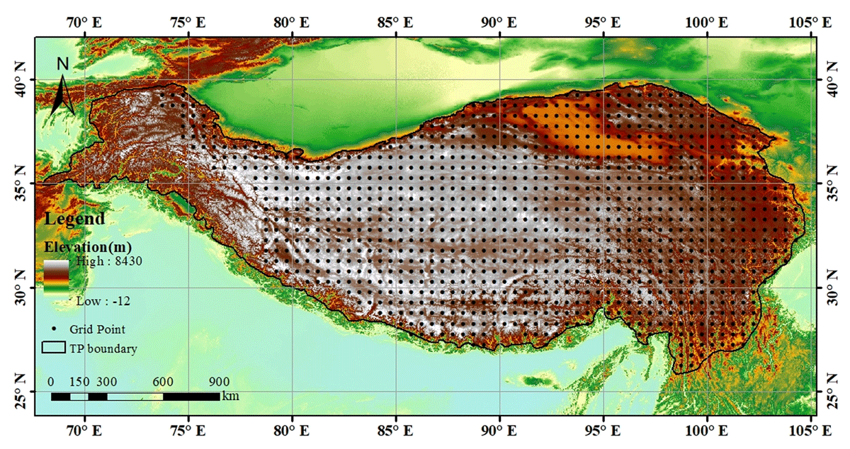
Figure 1
Geographical coverage of the study area and CMIP6 0.5° × 0.5° grid points (black dots).
Table 2
The information of the selected CMIP6 models in this study.
| NUMBER | MODEL NAME | MODELING CENTER | RESOLUTION |
|---|---|---|---|
| (LONGITUDE × LATITUDE) | |||
| 1 | ACCESS-CM2 | Commonwealth Scientific and Industrial Research Organisation, Australia | 1.875° × 1.25° |
| 2 | ACCESS-ESM1-5 | Commonwealth Scientific and Industrial Research Organisation, Australia | 1.875° × 1.2143° |
| 3 | AWI-CM-1-1-MR | Alfred Wegener Institute, Helmholtz Centre for Polar and Marine Research, Germany | 0.9375° × 0.9375° |
| 4 | BCC-CSM2-MR | Beijing Climate Center and China Meteorological Administration, China | 1.125° × 1.125° |
| 5 | CanESM5 | Canadian Centre for Climate Modeling and Analysis, Canada | 2.8125° × 2.8125° |
| 6 | CanESM5-CanOE5 | Canadian Centre for Climate Modeling and Analysis, Canada | 2.8125° × 2.8125° |
| 7 | CNRM-CM6-1 | National Centre for Meteorological Research and European Centre for Research and Advanced Training in Scientific Computation, France | 1.40625° × 1.40625° |
| 8 | CNRM-CM6-1-HR | National Centre for Meteorological Research and European Centre for Research and Advanced Training in Scientific Computation, France | 0.5° × 0.5° |
| 9 | CNRM-ESM2-1 | National Centre for Meteorological Research and European Centre for Research and Advanced Training in Scientific Computation, France | 1.40625° × 1.40625° |
| 10 | EC-Earth3-Veg | EC-Earth consortium, Europe | 0.703125° × 0.703125° |
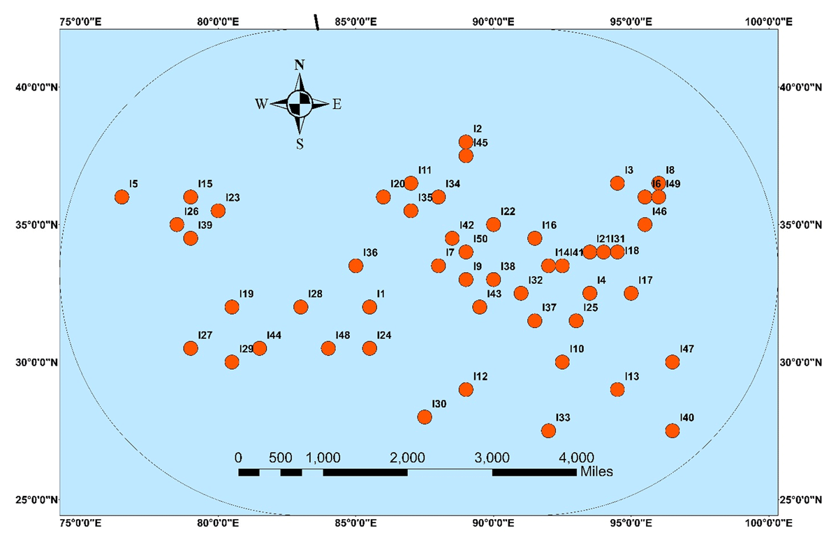
Figure 2
Spatial distribution fifty random location scattered over Tibet Plateau.
6. Results and discussion
6.1. Inference of Forecastable Component analysis on multi model climate model of CMIP-6
The crucial aspect in multivariate time series analysis is to reduce the dimension of data by keeping the forecasting characteristics. This section is related to the implication of FCA in dimension reduction context. Here, we present and discuss the results associated with the application of FCA on the multivariate time series data set of 23 climate simulated models of CMIP-6. The main objective of using FCA is to achieve aggregate time-series data that have inherited forecastability features for drought forecasting. In computation and inference, the research employed ForeCA (Goerge, 2016a).
Figure 3 shows the graphical summary of FCA on the time series data of 23 climate models at one random grid point of Tibet Plateau. At this grid point, we have assessed that the first component has 77.08% forecasting ability. Forecasting features are inherently time-limited. Therefore, reducing prediction errors is always a difficult task. In general, drought is complex and difficult to predict. However, the high forecastibility make sure the more prediction accuracy under the proposed index. Table 3 provides the values of Ω for the reaming components. Here, the highest values of Ω for the first components reveal its excellent forecasting ability. In other words, the highest value of Ω of the first component shows that it has is more forecastable.
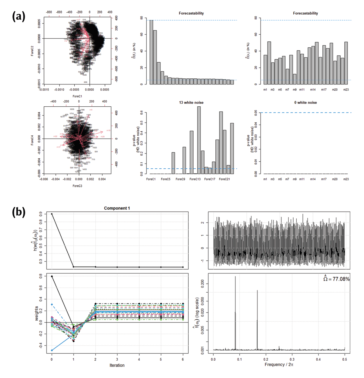
Figure 3
a) Biplots, forecastibility and b) summary of single FPC.
Table 3
Values of Omega against each components.
| COMPONENTS | OMEGA (Ω) |
|---|---|
| ForeC1 | 77.08283 |
| ForeC2 | 64.98184 |
| ForeC3 | 26.62885 |
| ForeC4 | 15.64948 |
| ForeC5 | 10.16605 |
| ForeC6 | 8.119885 |
| ForeC7 | 7.546159 |
| ForeC8 | 7.281088 |
| ForeC9 | 7.117616 |
| ForeC10 | 7.077022 |
| ForeC11 | 6.888564 |
| ForeC12 | 6.882761 |
| ForeC13 | 6.791538 |
| ForeC14 | 6.623308 |
| ForeC15 | 6.611346 |
| ForeC16 | 6.607055 |
| ForeC17 | 6.302802 |
| ForeC18 | 6.256745 |
| ForeC19 | 6.184776 |
| ForeC20 | 6.074139 |
| ForeC21 | 5.896357 |
| ForeC22 | 5.723812 |
| ForeC23 | 5.685728 |
Similarly, the FCA algorithm is performed for all the grid points of Tibet Plateau. Figure 4 shows the spatial distribution of Ω. It is observed that only one or two grid points have a significantly small value of Ω (<50). In addition, the range Ω lies between 50–60 covers a comparatively small area. However, a large number of portion of grid points have Ω greater than 60. In dimension reduction context, these inferences validate the use of FCA for increasing the forecastability of drought features under multiple climate models.
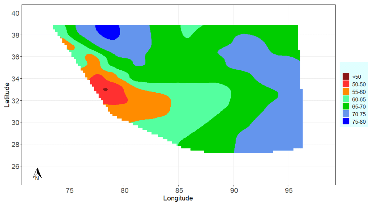
Figure 4
Spatial distribution of Omega (Ω).
6.2. Estimation of MMFSDI and SPI
After obtaining the time series data of the first component of FCA for each grid point, we have obtained the MMFSDI data by standardizing the CDF of L-CGMD. We have followed this new procedure due to Ali et al., (2021a, 2021b). For comparison, SPI time series data is obtained by averaging all the historical simulation models, accordingly. This section explores quantitative and graphical results related to the estimation of MMFSDI and SPI. For one random selected grid point, Figure 5 shows the density plots corresponding with q-q plots observed on the precipitation (averaged of all the selected climate models) and the first component of FCA at a one-month time scale. Here, we have observed the BIC value for MMFSDI (BIC = –4357.048) is comparatively low than for the estimation of SPI (BIC = –4003.55). This shows that the data of the first component of FCA is more accurately describable than simple model averaging. Resultantly, we can say that MMFSDI is more accurate than SPI. Similar results have been found for the rest of the time scale (see Table 4). To check the consistency between SPI and MMFSDI, Figure 6 is prepared to show the temporal behavior of MMFSDI and SPI. While the correlation analysis reveals that MMFSDI is strongly correlated with SPI (see Figure 7). This consistency leads towards the endorsement of MMFSDI as an alternative drought indicator.
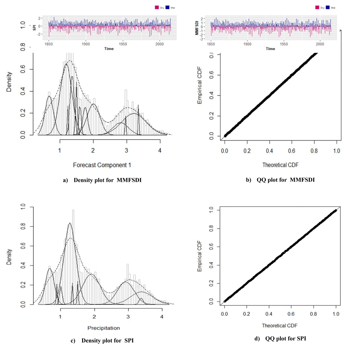
Figure 5
Density and qq plot of KCGMD for SPI and MMFSDI at one month time scale.
Table 4
BIC of KCGMD for SPI and MMFSDI.
| TIME SCALES | SPI | MMFSDI |
|---|---|---|
| Scale 1 | –4003.55 | –4357.048 |
| Scale 6 | –8614.13 | –9084.659 |
| Scale 9 | –7977.962 | –8446.784 |
| Scale 12 | –4295.112 | –4548.289 |
| Scale 24 | –5609.977 | –5905.589 |
| Scale 48 | –6740.838 | –6921.417 |
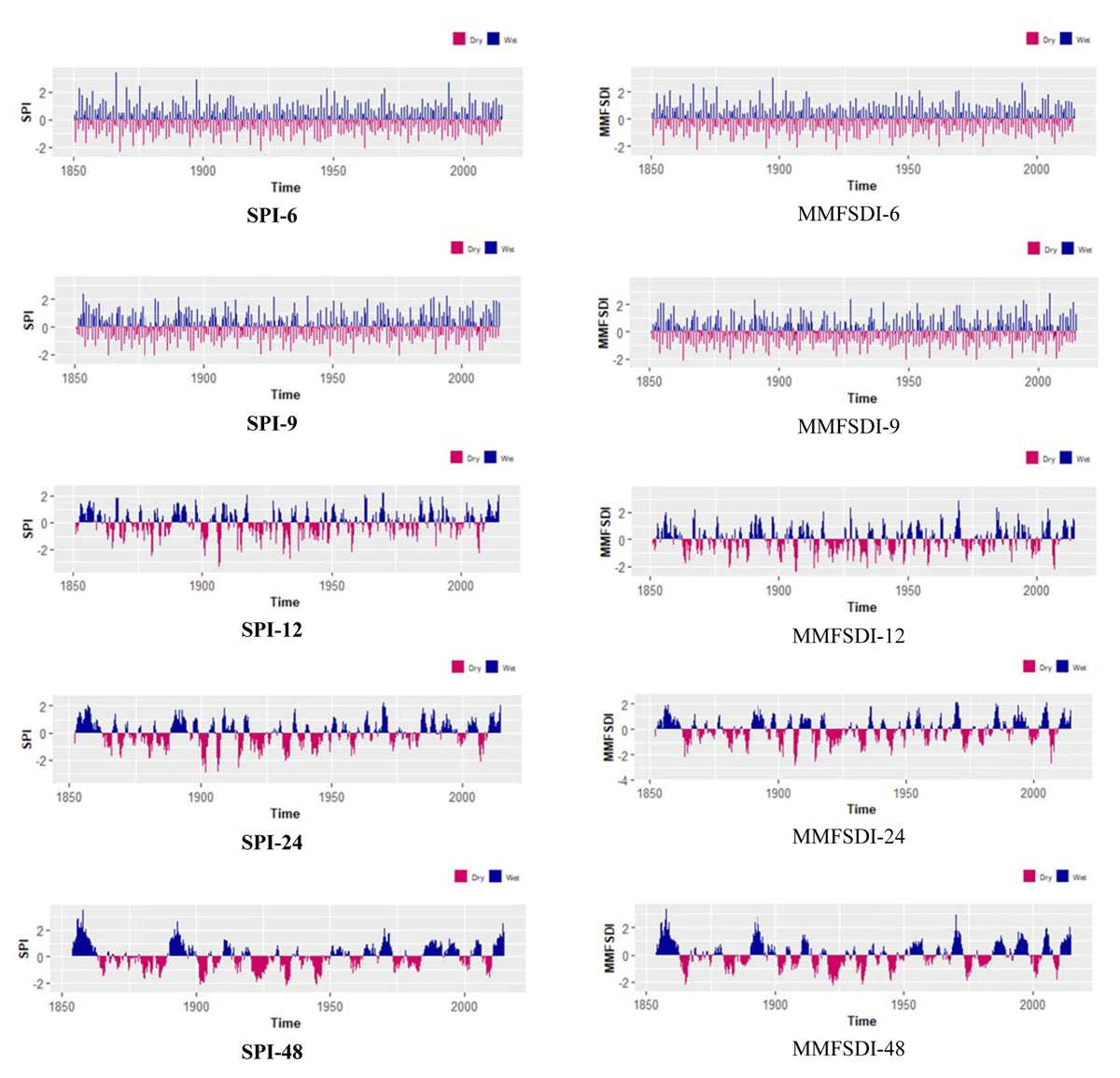
Figure 6
Temporal behaviour of SPI and MMFSDI in various time scale.
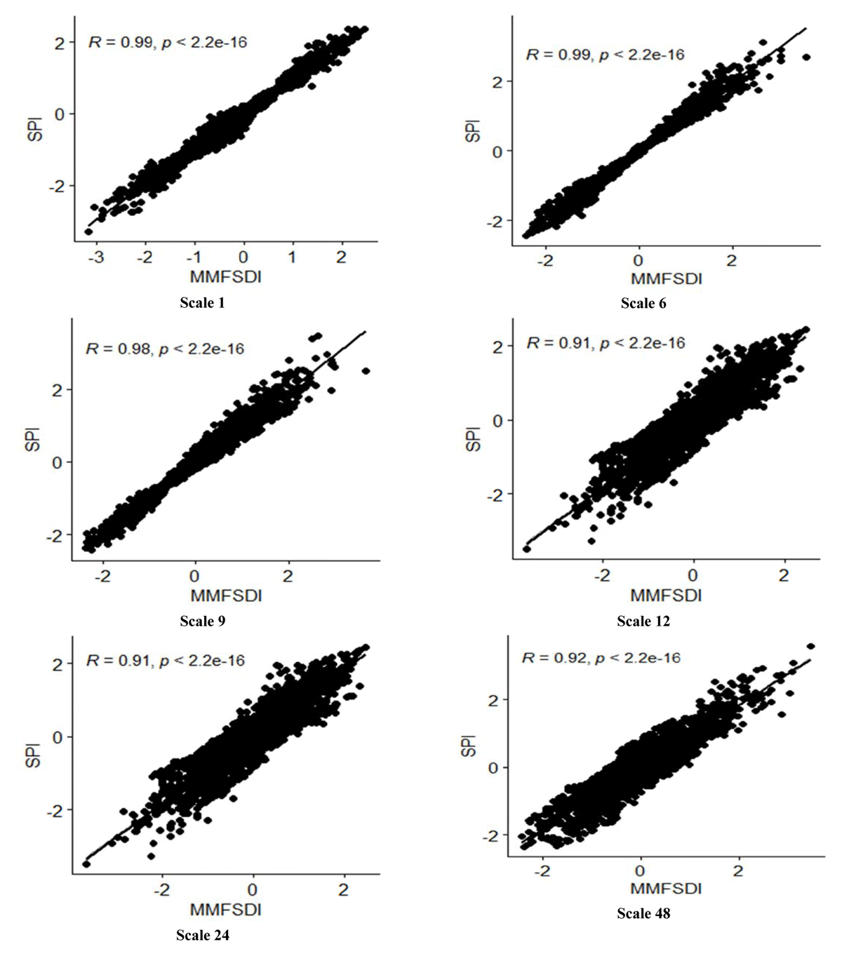
Figure 7
Correlation anaysis between SPI and MMFSDI in various time scales.
To assess that MMFSDI is more forecastable than SPI, the next section presents inferences related to ARIMA and ANN modeling.
6.3. Comparative evaluation
This section presents the results associated with comparative evaluation of the proposed ensemble approach with model averaging based drought index. Here, the forecasting efficiency of MMFSDI is compared with SPI using performing matrices of ARIMA and ANN techniques. In this article, the results related to the implications of ARIMA and ANN have been provided for one random grid point. The remaining results of all other grid points are in accordance with that random point. According to standard practice, the implications of ARIMA and ANN have consisted of training and testing phase. The training phase is employed for the estimation of model parameters and assessment of prediction accuracy, while the testing phase describes the forecasting accuracy. The two models ARIMA and NN are executed for each time scale of MMFSDI and SPI, separately. To do this, this research has employed forecast and nnet packages of R statistical software.
In both the training and testing phase, the performance assessment criterion of ARIMA and ANN have analogous evaluation (see Table 5). In training phase, ARIMA gives the comparative low value of RMSE (0.580) and MAE (0.445) for MMFSDI than SPI (RMSE = 0.760, MAE = 0.601) at one-month time scales. Accordingly, the similar quantitative assessment of performing matrices in the testing phase proves that MMFSDI is more predictable than SPI at month time scale. Although, some inadmissible quantitation in performing matrices have been observed at a 24-month time scale. However, the forecasting ability of MMFSDI in most of the time scales is comparatively high. Contrary to ARIMA, the performing matrices in both the training and testing phase under ANN models show that the forecasting ability of MMFSDI is high from SPI in all time scales. Furthermore, the quantitation deviation in RMSE and MAE at the training and testing phase between ARIMA and ANN shows that ANN is more appropriate than ARIMA. Hence, these results substantiate that MMFSDI is a more appropriate indicator than SPI for forecasting future values of drought under multiple climate models.
Table 5
Performance assessment of MMFSDI over SPI.
| TRAINING | TESTING | |||||
|---|---|---|---|---|---|---|
| TIME SCALES | TECHNIQUES | INDEX | RMSE | MAE | RMSE | MAE |
| Scale 1 | ARIMA | SPI | 0.760 | 0.601 | 0.962 | 0.774 |
| MMFSDI | 0.580 | 0.445 | 0.737 | 0.555 | ||
| MLP | SPI | 0.302 | 0.233 | 1.010 | 0.831 | |
| MMFSDI | 0.191 | 0.145 | 0.752 | 0.588 | ||
| Scale 6 | ARIMA | SPI | 0.474 | 0.341 | 1.089 | 0.885 |
| MMFSDI | 0.229 | 0.172 | 0.655 | 0.491 | ||
| MLP | SPI | 0.163 | 0.112 | 0.650 | 0.540 | |
| MMFSDI | 0.115 | 0.078 | 0.399 | 0.307 | ||
| Scale 9 | ARIMA | SPI | 0.438 | 0.331 | 1.658 | 1.349 |
| MMFSDI | 0.396 | 0.317 | 1.106 | 0.871 | ||
| MLP | SPI | 0.150 | 0.108 | 0.826 | 0.644 | |
| MMFSDI | 0.116 | 0.085 | 0.440 | 0.335 | ||
| Scale 12 | ARIMA | SPI | 0.346 | 0.266 | 0.683 | 0.548 |
| MMFSDI | 0.343 | 0.258 | 1.398 | 1.138 | ||
| MLP | SPI | 0.225 | 0.173 | 1.564 | 1.222 | |
| MMFSDI | 0.223 | 0.171 | 0.941 | 0.631 | ||
| Scale 24 | ARIMA | SPI | 0.227 | 0.173 | 0.497 | 0.450 |
| MMFSDI | 0.241 | 0.179 | 1.167 | 1.000 | ||
| MLP | SPI | 0.163 | 0.125 | 1.339 | 0.903 | |
| MMFSDI | 0.162 | 0.121 | 0.406 | 0.324 | ||
| Scale 48 | ARIMA | SPI | 0.153 | 0.108 | 1.250 | 1.102 |
| MMFSDI | 0.141 | 0.106 | 1.135 | 1.121 | ||
| MLP | SPI | 0.151 | 0.107 | 1.041 | 0.904 | |
| MMFSDI | 0.143 | 0.106 | 0.917 | 0.851 | ||
7. Summary and conclusion
Accurate and efficient ensemble procedures of historical simulations of various climate models are essential for drought monitoring. The appropriate choice for selecting an ensemble depends on the certain quantitative characteristics such as low biases and forecasting errors. This papers provides a novel way to ensemble climate models for drought forecasting. Here, a new drought indicator- the Multivariate Multi-Scaler Forecastable Standardized Drought Index (MMFSDI) has been proposed. Contrary to other drought indices, the distinctive ability of MMFSDI is the inherited forecasting feature. This is because the standardized values of MMFSDI are based on the first component of FCA. To assess the performance of MMFSDI, the paper included statistical inferences based on 50 random grid points of the Tibet Plateau. Here, historical simulated data of 23 climate models of CMIP-6 is used to obtain MMFSDI. While the comparative assessment is based on SPI under ANN and ARIMA models. Under both forecasting algorithms, outcomes associated with this research show that MMFSDI has an inherited ability to forecast drought under multiple climate models. In summation, the research provides an alternate approach for an ensemble of climate models for analyzing and forecasting drought features. Thus, this research strengthens the drought forecasting module by providing a new multiple climate simulated data based drought monitoring indicator.
Date Accessibility Statements
All the data were analyzed using R software. The data and code used to support the findings of this study are available from the corresponding author upon request.
Ethics and Consent
The manuscript is prepared in accordance with the ethical standards of the responsible committee on human experimentation and with the latest (2008) version of the Helsinki Declaration of 1975.
Funding Information
The authors are very grateful to the Natural Science Foundation of Jiangsu Province, China (BK20210369).
Competing Interests
The authors have no competing interests to declare.
Author Contributions
All authors have equal contributions.