Selecting CMIP6 Models for Future Arctic Storylines Using a Novel Performance Score

1 Introduction

Any application of modeled climate data should be supported by an evaluation of the basic performance of the model, that is, how well it simulates the observed climate, for the variables, regions, and seasons of interest. When using multi-model ensembles such as the global climate model simulations from the Coupled Model Intercomparison Project phase 6 (CMIP6; Eyring et al., 2016a), it can be necessary to identify models that do not perform as well as the rest of the ensemble and that warrant additional investigation or even exclusion from further analysis. This is particularly relevant when it is not desirable or even permissible to use the entire ensemble of models and a subset must be chosen instead. An example is dynamical downscaling of CMIP6 models, as it is computationally prohibitive to consider downscaling the full CMIP6 ensemble with a regional climate model. Another is identifying individual CMIP6 models that are most representative of specific storylines of future climate change (Williams et al., 2024). While the final model selection tends to be subjective, the process can benefit from being guided by objective evaluations.

A number of methods and tools for evaluating the simulated climate of multi-model ensembles already exist (e.g., Eyring et al., 2019), ranging in complexity from simple online applications like GCMeval (Parding et al., 2020) to more comprehensive evaluation systems like the Earth System Model Evaluation tool (ESMValTool; Eyring et al., 2016b; Righi et al., 2020). Methods can be based on basic statistical metrics like mean relative error (e.g., Gleckler et al., 2008), normalized error variance (e.g., Reichler and Kim, 2008), and root-mean-square error (RMSE) that has been normalized by observational uncertainty (e.g., Karpechko et al., 2010), or more complex frameworks like empirical orthogonal functions (e.g., Ashfaq et al., 2022; Hannachi, 2021), common empirical orthogonal functions (e.g., Benestad et al., 2023; Hannachi et al., 2022; Hannachi, 2021; Sengupta and Boyle, 1998), atmospheric circulation-type statistics (e.g., Brands, 2022), or clustering (e.g., Samantaray et al., 2023; Yokoi et al., 2011). Furthermore, there are specialized diagnostics like the Taylor diagram (Taylor, 2001), which can summarize multiple metrics in one single plot. Each of these scores and diagnostics offers different valuable insights into the climate models and the ensembles, but each also has its limitations. Condensing model evaluation into one single metric remains challenging, although great progress has been made to combine different diagnostics to produce a single-value performance score for each model (e.g., Gleckler et al., 2008; Hu et al., 2022; Karpechko et al., 2010; Reichler and Kim, 2008; Samantaray et al., 2023).

Here, we define a novel and simple score for comparing data from multiple climate models to reference data from reanalysis and gridded observations that is based on average normalized RMSE (NRMSE) for multiple variables, the RMSE-based relative performance score (RRPS). Unlike previous studies, we normalize the RMSE values so that they vary between 0 and 1 for all variables. This simplifies the interpretation of the results as it allows for all variables to exert a comparable influence on the score. By design, the score provides a measure of the relative model performance within the ensemble and facilitates identifying models that stand out from the rest of the ensemble.

We demonstrate the benefits and limitations of the score by using it to aid the selection of a single CMIP6 model or a set of CMIP6 models to represent storylines of Arctic climate change previously identified by Levine et al. (2024). Storylines can be defined as physically plausible potential pathways of future climate change (Zappa and Shepherd, 2017). The storylines methodology provides a way of examining several possible future outcomes with distinctly different climatological characteristics in parallel. Levine et al. (2024) showed that during the extended summer season (May, June, July, August, September, and October; MJJASO), large parts of the Arctic inter-model spread can be explained by inter-model differences in two predictors: Barents-Kara Sea surface warming and Arctic amplification. From this, they derived four storylines of summer Arctic climate based on the strength (weak or strong) of these predictors.

To establish a set of CMIP6 models to represent each of the four storylines defined in Levine et al. (2024), we first identify a set of models that are similar to the storylines in terms of their Barents-Kara Sea warming and Arctic amplification and compute an estimate of this similarity. Then we use the score to evaluate the relative present-day performance of the models considering four impact-relevant variables used in Levine et al. (2024): near-surface temperature (tas), total (large-scale and convective) precipitation rate (pr), 850-hPa air temperature (ta850), and 850-hPa zonal wind (ua850). Finally, we identify the models most suitable for representing the storylines by combining the similarity estimate and the scores.

In what follows, we first provide an overview of the data used in Section 2 and a detailed description of the RRPS methodology in Section 3. We summarize pertinent information from Levine et al. (2024), introduce a similarity estimate, and use this estimate to establish a list of candidate models for each storyline in Section 4.1. We then consider the similarity estimate in combination with scores for Arctic extended summer in section 4.2 and in combination with scores for a more comprehensive set of seasons and regions in Section 4.3. Finally, we summarize and discuss our findings in Section 5.

2 Data

We use data from CMIP6 historical experiments (Eyring et al., 2016a) from 50 models (see appendix A for a complete list). The models were selected based on: (1) whether they had performed the CMIP6 historical and the shared socioeconomic pathway scenario that corresponds to a 8.5 W m^-1 increase in radiative forcing by the end of the 21st century (SSP5-8.5; O’Neill et al., 2016); and (2) whether all necessary fields were available at the Earth System Grid Federation (ESGF) at the time of the data retrieval: monthly tas, pr, zonal wind (ua), air temperature (ta), and surface pressure (ps). For ua and ta, we extract the 850-hPa level (ua850 and ta850). While ps is not explicitly included in the score, it is used to filter out below-surface grid points from the 850-hPa fields for consistency across the models (this is needed as some models extrapolate and others assign missing/fill values to sub-surface grid points). Hence, we consider four variables for the score: tas, pr, ua850, and ta850.

To verify the models, we use reference data from the 5th generation of the European Center for Medium-Range Weather Forecasts’ Reanalysis (ERA5; Hersbach et al., 2020) for ps, tas, ta850, and ua850 (Hersbach et al., 2019a, b) and from the Global Precipitation Climatology Project precipitation analysis (GPCP; Adler et al., 2003) for pr (Adler et al., 2016). We use years 1985–2014 in all cases.

3 The RRPS Methodology

The RRPS quantifies the model’s ability to simulate the historical climate for the selected variables as a single value, and is defined as the average NRMSE taken over a set of variables. We base the score on RMSE as it is not affected by cancellation of positive and negative errors (like the bias) and emphasizes large errors. Here, the score is based on tas, pr, ta850, and ua850. We consider both annual and seasonal scores. Below, we outline the procedure for computing the scores step by step.

1. As an initial step, we bilinearly interpolate all data to a common 1° × 1° grid in the horizontal.

2. We then compute monthly climatologies, that is, multi-year mean values computed separately for each month of the year.

3. To ensure consistency across the models, we mask out sub-surface grid points (i.e., in areas of high elevation) in ua850 and ta850 using ps.

4. The RMSE values are computed as the root of the squared differences between the monthly climatological values from the CMIP6 models and the relevant reference data sets for the same time period, 1985–2014. For a variable X, model c, month m, and reference data set denoted REF, we compute the RMSE values separately for each zonal grid point i and meridional grid point j:

   1

   ${\text{RMSE}}_{X,c,m,i,j}=\sqrt{{\left(X_{c,m,i,j}–X_{\mathit{\text{REF}},m,i,j}\right)}^2}$

5. To account for variations of grid-cell area with latitude, RMSE values are spatially averaged using a standard cosine weighting:

   2

   ${\text{RMSE}}_{X,c,m}=\frac{{\sum }_{i,j}\cos ({\varphi }_j)\times {\text{RMSE}}_{X,c,m,i,j}}{{\sum }_{i,j}\cos ({\varphi }_j)}$

   where $\varphi$ is latitude.

6. We average the RMSE values temporally, using all months for annual values or a subset for seasonal values, and then normalize them so that they vary between 0 (for the best model) and 1 (for the worst model) following the approach used by Ashfaq et al. (2022) to normalize the absolute error (their equation 1):

   3

   ${\text{NRMSE}}_{X,c}=\frac{{\text{RMSE}}_{X,c}–\mathit{\text{min}}({\text{RMSE}}_{X,c_{\mathit{\text{all}}}})}{\max ({\text{RMSE}}_{X,c_{\mathit{\text{all}}}})–\min ({\text{RMSE}}_{X,c_{\mathit{\text{all}}}})}$

   where the subscript c_all indicates that all models are used.

7. Finally, the RRPS for each model (${\text{RRPS}}_c$) is computed as the average NRMSE across the variables X:

   4

   ${\text{RRPS}}_c=\frac{1}{N}\sum _{X=1}^{X=N}{\text{NRMSE}}_{X,c}$

An advantage of this normalization technique is that the NRMSE values vary within the same range (0 to 1) for all variables, meaning that the importance of all variables is more comparable than if we use the non-normalized RMSE. The score has the same range as the NRMSE, with low scores being favorable, indicating smaller errors than the other models, and higher values indicative of larger errors. The top score of 0 is only obtained if the same model is consistently the best performing model ($\text{NRMSE}=0$) for all variables and the worst score of 1 is only obtained if the same model has the largest relative errors in the ensemble ($\text{NRMSE}=1$) for all variables. Another advantage of the normalization is that it easily allows for different variables to be assigned weights if necessary.

We compute the score separately for six geographical regions: the whole globe, the tropics (15°S–15°N), Northern Hemisphere (NH) mid-latitudes (15°N–55°N), Southern Hemisphere (SH) mid-latitudes (15°S–55°S), Arctic (55°N–90°N), and Antarctic (55°S–90°S). One should note that our somewhat broad definition of the Arctic is chosen for consistency with Levine et al. (2024) and includes large land areas with boreal forest, which have a significantly different climate (e.g., more precipitation, warmer summers) than the ocean- and sea-ice-dominated central Arctic. For both the Arctic and Antarctic, the placement of the equatorward border means that it better captures the jet streams and storm tracks than other more restrictive definitions of the polar regions.

We consider the annual and seasonal scores. Our main focus is on the extended NH warm season (MJJASO), as this season was used to construct the storylines in Levine et al. (2024). However, we also include the four standard three-month seasons: December, January, and February (DJF), March, April, and May (MAM), June, July, and August (JJA), and September, October, and November (SON).

Next, we identify candidate models from the CMIP6 ensemble to represent the storylines from Levine et al. (2024) and provide an estimate of how similar the candidate models are to the storylines. Then, we combine these similarity estimates with the scores to produce an estimate of the overall fit for each candidate model, and use this as a basis for selecting models to represent the storylines, first for Arctic MJJASO (Section 4.2) and then for the full set of regions and seasons (Section 4.3).

4 Results

4.1 Arctic storylines of climate change

Storylines are physically plausible scenarios of future climate change, statistically derived from an ensemble of climate model projections, which are organized according to the magnitude of the projected changes in two or more remote drivers (e.g., Arctic amplification) that strongly influence the spatial pattern of the climate response (Zappa and Shepherd, 2017). Levine et al. (2024) applied the storylines methodology to find potential future pathways of Arctic climate change based on the CMIP6 historical and SSP5-8.5 scenario from an ensemble of CMIP6 models. An extended NH warm season MJJASO was defined because of its importance for societal and ecological impacts of climate change, that is, Arctic wildfires and permafrost thaw, which are especially pronounced during the summer (e.g., Chadburn et al., 2017; Masrur et al., 2018; McCarty et al., 2021). Using a multivariate linear regression framework, Levine et al. (2024) regressed the pattern of change in tas, ua850, pr, and sea-ice fraction onto two predictors that were found to explain most of the inter-model variability: Barents-Kara Sea warming and lower-tropospheric Arctic warming. Based on this, four storylines of future Arctic climate change were identified (see also Table 1): storyline A, weak Arctic amplification and strong Barents-Kara Sea warming; storyline B, strong Arctic Amplification and strong Barents-Kara Sea warming; storyline C, weak Arctic amplification and weak Barents-Kara Sea warming; and storyline D, strong Arctic Amplification and weak Barents-Kara Sea warming.

Table 1

Overview of Arctic storylines (A–D) and CMIP6 candidate models. The storylines are listed in column 1 and the two predictors the storylines are based on, the strength (+/–) of the Arctic amplification (ArcAmp+/–) relative to the multi-model mean, and the strength (+/–) of the Barents-Kara Sea warming (BKWarm+/–) relative to the multi-model mean, are listed in columns 2 and 3. The CMIP6 candidate models are listed in column 4, their abbreviations (abbr.) in column 5, the realization that is closest to the storyline point in the predictor-phase diagram (Figure 1) in column 6, and the Euclidean distance (ED) between the model/realization and the storyline point in the predictor-phase diagram in column 7. We omit FIO-ESM-2-1 (r1i1p1f1; ED = 0.73) from storyline A due to technical issues and EC-Earth3 (r112i1p1f1; ED = 0.69) from storyline B as ps was not available. Note that the models are ranked by the Euclidean distance for each storyline.

STORYLINE	PREDICTOR 1	PREDICTOR 2	CANDIDATE MODEL	ABBR.	REALIZATION	ED
A	ArcAmp–	BKWarm+	CNRM-CM6-1	A1	r1i1p1f2	0.38
			CIESM	A2	r1i1p1f1	0.44
			MPI-ESM1-2-LR	A3	r17i1p1f1	0.48
			CNRM-ESM2-1	A4	r1i1p1f2	0.62
B	ArcAmp+	BKWarm+	MIROC-ES2L	B1	r8i1p1f2	0.12
			MIROC6	B2	r23i1p1f1	0.17
			HadGEM3-GC31-LL	B3	r3i1p1f3	0.73
			UKESM1-0-LL	B4	r8i1p1f2	0.74
C	ArcAmp–	BKWarm–	CESM2-WACCM	C1	r1i1p1f1	0.09
			GISS-E2-1-H	C2	r5i1p1f2	0.11
			CAMS-CSM1-0	C3	r1i1p1f1	0.14
			GISS-E2-1-G	C4	r3i1p5f1	0.26
			MCM-UA-1-0	C5	r1i1p1f2	0.38
			CAS-ESM2-0	C6	r3i1p1f1	0.55
D	ArcAmp+	BKWarm–	NorESM2-MM	D1	r1i1p1f1	0.16
			KACE-1-0-G	D2	r1i1p1f1	0.66

Building on the work of Levine et al. (2024), we identify models from the CMIP6 ensemble that are representative of the different storylines. We start by evaluating the model’s ability to represent the Arctic storylines in terms of their projected strengthening of Arctic amplification and surface warming of the Barents-Kara seas (Figure 1). For each storyline (blue and red dots in Figure 1), we define a region around it, constrained by the isoline where the Euclidean distance from the storyline point is 0.75 in predictor space, and consider models that fall within this region to be candidate models for that storyline. This threshold is selected to ensure that the candidate models are close to the storyline point and that all storylines have multiple candidate models. For models with more than one realization, we consider the realization that is closest to the storyline point. A detailed overview of the candidate models and realizations we use for the different storylines is provided in Table 1.

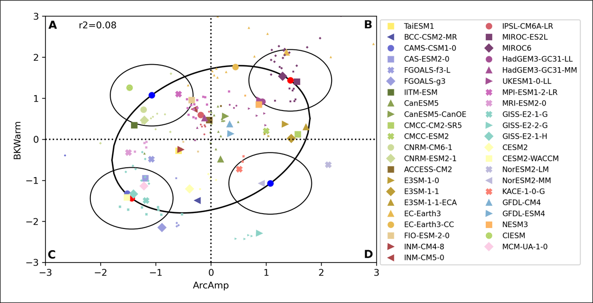
Figure 1

Having defined a set of candidate models for each storyline, we next quantify the representativeness (or similarity) of the candidate models by computing the Euclidean distance between the location of the candidate models and the relevant storyline point (Figure 1). The Euclidean distances for all candidate models are given in Table 1. Results show that storylines B, C, and D all have at least one candidate model that is very close to the storyline point, with the closest models found at an Euclidean distance of 0.12 (MIROC-ES2L), 0.09 (CESM2-WACCM), and 0.16 (NorESM2-MM) from the storyline points. For storyline A, the four candidate models are all found somewhat further away, with the smallest distance being 0.38 (CNRM-CM6-1).

In what follows, we use the score described in Section 3 to assess the performance of the full set of CMIP6 models (Appendix A), with particular emphasis on the performance of candidate models relative to the other models in the ensemble. We then use the scores in combination with the Euclidean distance to select a single model or a set of models to represent each storyline. We start by considering the same region and season as Levine et al. (2024), namely the Arctic during MJJASO in Section 4.2.

4.2 Arctic extended summer

The Arctic MJJASO (non-normalized) RMSE values for tas, pr, ua850, and ta850 are shown in Figure 2. While most values are within one standard deviation of the multi-model mean (white cells), others deviate more (blue/red cells). It is clear that some models are characterized by values that are favorable (low) relative to the rest of the multi-model ensemble (blue cells), while others are characterized by more disadvantageous (higher) values (red cells). In some cases, the RMSE values can deviate from the multi-model mean by several standard deviations. The multi-model statistics (yellow cells at the bottom of the table) show that the mean and spread vary from variable to variable, with some variables being characterized by a more pronounced spread relative to the multi-model mean than others. The diversity between variables emphasizes the importance of normalizing the RMSE values before combining them into a single score. This is not only needed to achieve dimensionless numbers, but also prevents the score from being dominated by the presence of variables that are characterized by larger errors than the others, thus ensuring that all four variables exert a more comparable influence on the score. The inclusion of two temperature variables means that the combined influence of temperature on the score will be larger than that from precipitation or zonal wind. However, we opt to include both temperature fields for consistency with Levine et al. (2024) and because of the importance of these variables for impact assessments, as identified in Levine et al. (2024).

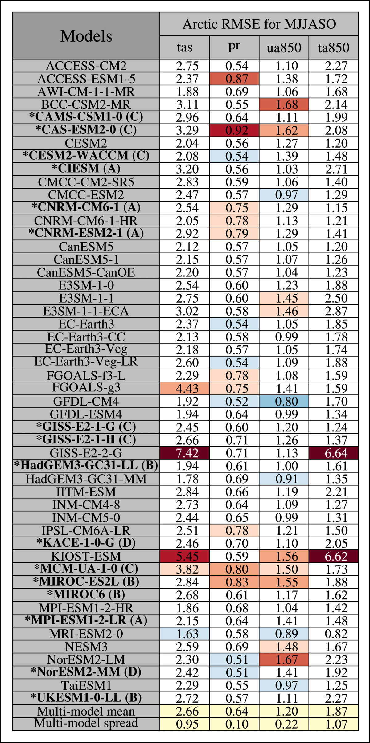
Figure 2

It is clear that models that perform substantially better than the multi-model mean in terms of Arctic MJJASO NRMSE (blue cells in Figure 3a) tend to perform well in terms of the score (b) and be placed in the upper part of the table, and vice versa. This is in line with the score being positively correlated with the NRMSE of the individual variables, with linear correlation coefficients of 0.79 for tas, 0.59 for pr, 0.73 for ua850, and 0.66 for ta850 (all values are significant at the p = 0.05 level following a Student’s t-test). The Arctic MJJASO scores range between 0.06 and 0.72. The best score is close to 0, meaning that the best-performing model (GFDL-CM4) performs well for all variables, although it does not consistently have the lowest NRMSE (which would give a score of 0). The worst (highest) score, however, is quite a bit better than the theoretical maximum value of 1, meaning that the relative performance of the model in question varies more from variable to variable; that is, no single model has the poorest relative performance for all four variables.

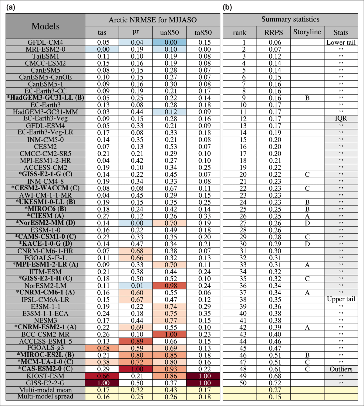
Figure 3

Storylines A, B, and C all have candidate models within the upper tail of the distribution (Figure 3b), defined as the range between the upper quartile (Q2) and Q2 plus 1.5 times the inter-quartile range (IQR). Storyline C also has a candidate model that is defined as an outlier (score exceeding Q2 plus 1.5 times the IQR). Only a single candidate model, HadGEM3-GC31-LL (a candidate for storyline B), places within the lower tail, defined as the range between the first quartile (Q1) and Q1 minus 1.5 times the IQR. The remaining candidate models are within the IQR.

In line with the score being a measure of relative model performance and the goal being to identify models with large errors compared to the rest of the multi-model ensemble, we consider candidate models with scores that are within the upper tail (including outliers) to be less preferable based on the relative performance for the variables, region, and season of primary interest.

To determine which model is most suited to represent the four storylines, we consider the Arctic MJJASO scores in combination with the Euclidean distance between the models and relevant storyline point in predictor space (Figure 1; Table 1). Specifically, we use the product of these two quantities to produce a measure of the overall fit for each model:

5

$\mathit{\text{fit}}={\text{RRPS}}_c(s,r)\times {\text{ED}}_c(s=\text{MJJASO},r=\text{Arctic})$

where fit is the overall fit, s is the season, and r is the region.

Hence, the overall fit combines the relative present-day model performance with the representativeness of the candidate models into a single value. Values for the overall fit, based on the Arctic MJJASO scores for the candidate models and the Euclidean distances from Table 1, are illustrated in Figure 4 (blue curves) and given in Table 2.

Table 2

Overview of MJJASO scores (RRPS) and overall fit for the whole (total) Arctic, Arctic land, and Arctic sea for the storyline candidate models. We use the model abbreviations defined in Table 1, repeated here for convenience: A1 (CNRM-CM6-1), A2 (CIESM), A3 (MPI-ESM1-2-LR), A4 (CNRM-ESM2-1), B1 (MIROC-ES2L), B2 (MIROC6), B3 (HadGEM3-GC31-LL), B4 (UKESM1-0-LL), C1 (CESM2-WACCM), C2 (GISS-E2-1-H), C3 (CAMS-CSM1-0), C4 (GISS-E2-1-G), C5 (MCM-UA-1-0), C6 (CAS-ESM2-0), D1 (NorESM2-MM), and D2 (KACE-1-0-G). For each storyline (column 1), the candidate-model abbreviations and their scores and overall fit for the whole Arctic, Arctic land, and Arctic sea are given in columns 2–4 and 5–7; the models are sorted by the score (columns 2–4) and overall fit (columns 5–7) with the best values on top.

STORYLINE	ARCTIC MJJASO RRPS			ARCTIC MJJASO OVERALL FIT
	TOTAL	LAND	SEA	TOTAL	LAND	SEA
A	A2 (0.25)	A2 (0.24)	A3 (0.23)	A2 (0.11)	A1 (0.10)	A2 (0.10)
	A3 (0.31)	A1 (0.27)	A2 (0.24)	A1 (0.13)	A2 (0.10)	A3 (0.11)
	A1 (0.34)	A3 (0.32)	A1 (0.35)	A3 (0.15)	A3 (0.15)	A1 (0.13)
	A4 (0.39)	A4 (0.33)	A4 (0.38)	A4 (0.24)	A4 (0.20)	A4 (0.23)
B	B3 (0.16)	B3 (0.15)	B2 (0.16)	B2 (0.04)	B2 (0.05)	B2 (0.03)
	B4 (0.23)	B4 (0.21)	B3 (0.17)	B1 (0.06)	B1 (0.07)	B1 (0.04)
	B2 (0.25)	B2 (0.29)	B4 (0.24)	B3 (0.12)	B3 (0.11)	B3 (0.12)
	B1 (0.51)	B1 (0.55)	B1 (0.36)	B4 (0.17)	B4 (0.16)	B4 (0.18)
C	C4 (0.22)	C4 (0.21)	C1 (0.20)	C1 (0.02)	C1 (0.02)	C1 (0.02)
	C1 (0.23)	C1 (0.22)	C4 (0.23)	C2 (0.04)	C2 (0.03)	C2 (0.04)
	C3 (0.28)	C3 (0.25)	C3 (0.28)	C3 (0.04)	C3 (0.04)	C3 (0.04)
	C2 (0.32)	C2 (0.30)	C2 (0.33)	C4 (0.06)	C4 (0.05)	C4 (0.06)
	C5 (0.51)	C6 (0.52)	C5 (0.40)	C5 (0.19)	C5 (0.21)	C5 (0.15)
	C6 (0.61)	C5 (0.54)	C6 (0.62)	C6 (0.33)	C6 (0.29)	C6 (0.34)
D	D1 (0.26)	D1 (0.21)	D1 (0.27)	D1 (0.04)	D1 (0.03)	D1 (0.04)
	D2 (0.29)	D2 (0.26)	D2 (0.31)	D2 (0.19)	D2 (0.17)	D2 (0.20)

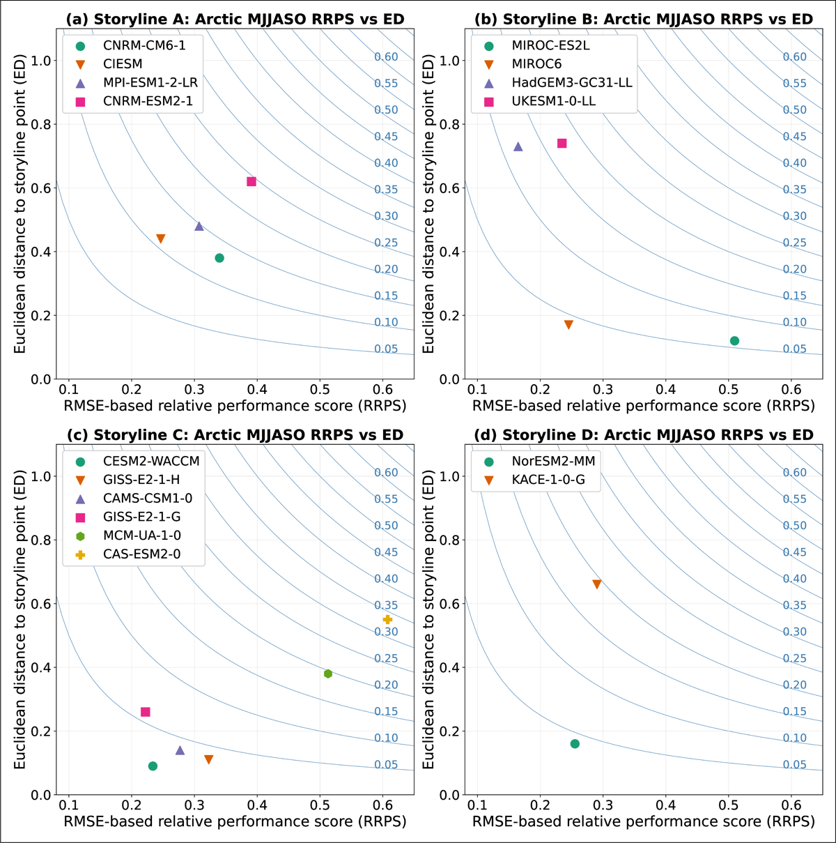
Figure 4

For storyline A, CIESM (brown downward-pointing triangle) is the best-performing candidate model, while CNRM-CM6-1 (green filled circle) is slightly more representative of the storyline, having a smaller Euclidean distance (Figure 4a). The overall fit is best (smallest) for CIESM, meaning that even though CIESM is somewhat further away from the storyline point, it has a slightly better overall fit due to its present-day performance (i.e, score) for Arctic MJJASO. The overall fit for CIESM is nevertheless very similar to that for CNRM-CM6-1 and MPI-ESM1-2-LR (purple upward-pointing triangle). These three candidate models for storyline A are more or less clustered together with both scores and Euclidean distance that are relatively similar; we therefore argue that they should all be considered acceptable choices for storyline A. The last candidate model, CNRM-ESM2-1, is also relatively similar to the other three, but is further away from the storyline point and has a score exceeding the 75th percentile (Figure 3).

For storyline B (Figure 4b), MIROC-ES2L (green filled circle) and MIROC6 (brown downward-pointing triangle) stand out from the other candidate models due to their small Euclidean distances. While HadGEM3-GC31-LL (purple upward pointing triangle) and UKESM1-0-LL (pink square) have the smallest and second smallest scores, they are both much further away from the storyline point. MIROC6 stands out as the best candidate, having a small Euclidean distance and a relatively low score, and the best overall fit. MIROC-ES2L has the second-best fit, but it also has one of the largest scores of all the models considered (0.51) with high relative errors for both pr and ua850 (Figure 3). To choose a second model for storyline B, one will have to prioritize between having a small Euclidean distance and a low score. As MIROC-ES2L is in the far end of the upper tail, we argue that HadGEM3-GC31-LL is preferable in this case.

For storyline C (Figure 4c), it is clear what while CESM2-WACCM (green filled circle) has the smallest Euclidean distance and the second lowest score, yielding the best overall fit, results are very similar for GISS-E2-1-H (brown downward-pointing triangle), CAMS-CSM1-0 (purple upward-pointing triangle), and GISS-E2-1-G (pink square); hence, all these four models are good representatives for storyline C. The other two candidate models are less preferable, as they have larger Euclidean distances and substantially larger scores.

Storyline D has only two candidate models, which are more or less indistinguishable in terms of the Arctic MJJASO score alone; the models are both within the IQR, with the relative performance of NorESM2-MM being slightly better than for KACE-1-0-G (RRPS 0.26 and rank 27 vs. RRPS 0.29 and rank 30; Figure 3). While it is difficult to select one over the other based on the score alone, Figure 4d clearly shows NorESM2-MM (green filled circle) is much closer to the storyline point than KACE-1-0-G (brown downward-pointing triangle), resulting in the best overall fit. NorESM2-MM is therefore the preferred choice for storyline D.

In summary, based on a combination of (1) how well the models represent the present-day state of four key variables in the Arctic during MJJASO and (2) the models’ proximity to the relevant storyline point in predictor space, we select CIESM, CNRM-CM6-1, and MPI-ESM1-2-LR to represent storyline A, MIROC6 to represent storyline B, CESM2-WACCM, GISS-E2-1-H, CAMS-CSM1-0, and GISS-E2-1-G to represent storyline C, and NorESM2-MM to represent storyline D. Storylines A and C both have multiple candidate models that are very similar, and we therefore recommend a set of models in these cases.

4.2.1 Performance for Arctic land and Arctic sea

Arctic climate change is associated with a wide range of impacts, some tied to processes over the land surface, such as wildfires and permafrost thaw (e.g., Chadburn et al., 2017; Masrur et al., 2018; McCarty et al., 2021), and others to changes in marine areas, such as sea-ice loss (e.g., Gulev et al., 2021; Screen and Simmonds, 2010). To assess how sensitive the model selection is to whether we base the score on NRMSE values for the whole Arctic, Arctic land, or Arctic sea, we compute the score and overall fit separately for these three regions (Table 2). Results show that the model with the best overall fit for the whole Arctic is generally also the model with the best fit for Arctic sea and Arctic land for all four storylines. For storyline A, CIESM has the best value for whole region and over the sea, while over land, CNRM-CM6-1 is marginally better (however, at two decimal precision, the overall fit is the same).

While this shows that our model selection for Arctic MJJASO holds regardless of whether we focus on the whole Arctic, Arctic land, or Arctic ocean, it is clear that the scores display some sensitivity to which part of the Arctic they are computed for. Next, we examine the sensitivity of the score further, comparing results for Arctic MJJASO to results from other regions and seasons. This will allow us to further investigate how robust our selection is, that is, whether the model selection based on the Arctic MJJASO scores still holds for other regions and seasons, or whether other candidate models are preferable.

4.3 Seasonal and regional sensitivity

Figure 5a compares the Arctic MJJASO scores (black dots in a) to the Arctic scores for the whole year and the four traditional three-month seasons (orange, blue, and red symbols), showing that the relative model performance can vary considerably throughout the year. The largest range (between the season with the worst and best score; numbers in the rightmost part of panel a) is found for GISS-E2-2-G, which has a range of 0.4 between the best-performing season (JJA; dark red square) and the worst (DJF; dark blue asterisk). There are no indications that the seasonal sensitivity increases linearly with the score, as large ranges are found for the models with low scores, small ranges are found for models with high scores, and vice versa.

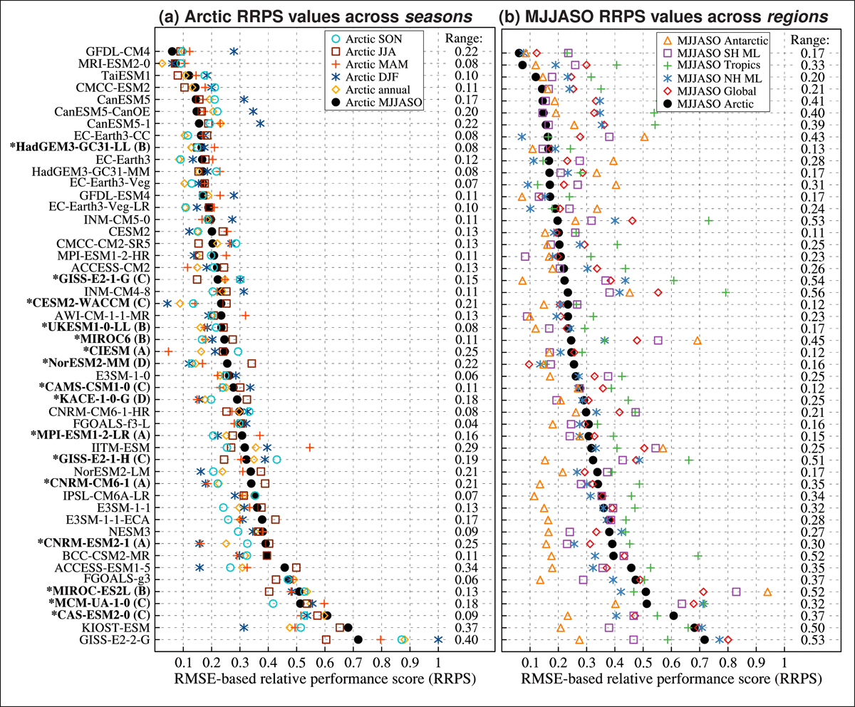
Figure 5

Interestingly, the relative performance of the models varies more across regions than across seasons. Comparing the seasonal variability (for Arctic scores across seasons; Figure 5a) to the regional variability (for MJJASO scores across regions; Figure 5b) clearly shows that the regional variability is larger. This is not only evident when comparing the regional spread for a single season (Figure 5b) to the seasonal scores for a single region (Figure 5a), but is a general result found when considering the seasonal spread for all regions (Figure 6a) to the regional spread for all seasons at the same time (Figure 6b).

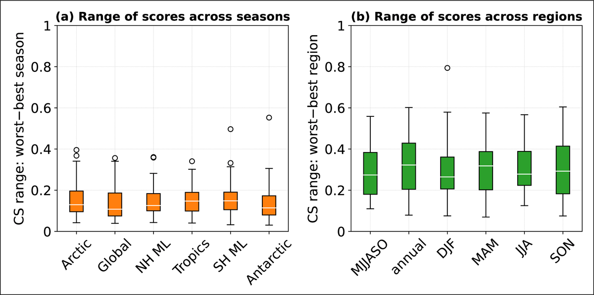
Figure 6

To further examine the regional sensitivity of the candidate models, we consider the MJJASO scores and ranks for these models for the different regions in Figure 7. While such an evaluation of the relative model performance is useful, it is important to keep in mind that both the scores and ranks are sensitive to the results for the other models, and that the sensitivity to the rest of the ensemble is stronger for the ranks. The score for an individual model is only affected by the subset of models that have the smallest or largest NRMSE value for one or more fields (equation 3). To find the ranking value of an individual model, on the other hand, the performance of the full set must be taken into account. Therefore, when comparing scores between regions for a single model, improved (lower) scores do not always translate to better (lower) ranking values, nor do worse scores always yield higher ranking values. For example, CNRM-ESM2-1 has a better score for the Antarctic (0.16) than for the SH mid-latitudes (0.23), but the ranking value is 17 in both cases. This happens because there are 16 better-performing models in both cases.

4.3.1 Storyline A

The models that were selected to represent storyline A based on the Arctic MJJASO scores, CNRM-CM6-1, CIESM, and MPI-ESM1-2-LR (Section 4.2), all have relatively consistent performance for the other regions (Figure 7a). Overall, the performance is best for CIESM, which has Arctic, global, NH mid-latitude, and Antarctic scores within the IQR (yellow cells) and tropical and SH mid-latitude scores below the 25th percentile (blue cells). CIESM is also the most consistent performer with a range of scores of 0.12. The second-best model is CNRM-CM6-1, which has scores within the IQR for every region except the Antarctic, where it is within the lower tail. MPI-ESM1-2-LR has scores within the IQR for all regions except the Antarctic, where it is ranked 40th with scores exceeding the 75th percentile (red cells). The last candidate model, CNRM-ESM2-1, is within the upper tail in the Arctic, but performs better for all other regions with scores within the IQR in all cases.

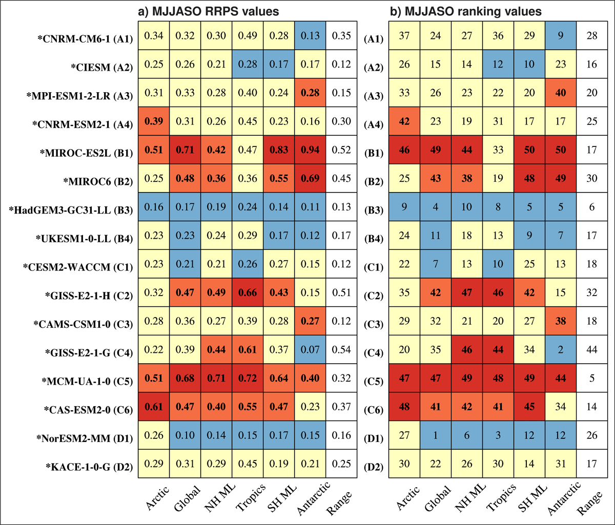
Figure 7

The overall fit for all seasons and regions (Figure 8a) shows that the CIESM (A2) is the overall best choice for storyline A, being either the best-performing model, or comparable to the best-performing model (e.g., in the Antarctic). To accentuate models with relatively good scores, we show markers for models with scores below the 75th percentile in strong colors (reds, blues, orange, and black), while markers for models whose scores exceed the 75th percentile are shown in light gray. The colors of the markers reveal that CIESM has no scores exceeding the 75th percentile.

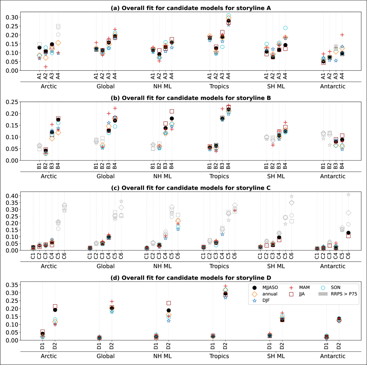
Figure 8

While the overall fit for the candidate models for storyline A is best for CIESM, values for CNRM-CM6-1 and MPI-ESM1-2-LR are largely similar. CNRM-ESM2-1, however, tends to have slightly higher values, particularly in the tropics, and has Arctic scores exceeding the 75th percentile during MJJASO, JJA, and SON (gray markers).

4.3.2 Storyline B

MIROC6, the selected model for storyline B based on the Arctic MJJASO results (Section 4.2), consistently performs worse for the other regions, with MJJASO scores (Figure 7a) exceeding the 75th percentile for the globe, NH mid-latitudes, SH mid-latitudes, and the Antarctic, with the latter furthermore being an outlier. Similarly, the MJJASO scores for MIROC-ES2L exceed the 75th percentile for every region except the tropics, with the global, SH mid-latitude, and Antarctic scores being outliers. This suggests that when considering other regions than the Arctic, it is preferable to use one of the three other candidate models for storyline B, even though they all have larger distances to the storyline point (Table 1). Based on the MJJASO scores for the six regions (Figure 7a), HadGEM3-GC31-LL and UKESM1-0-LL are the best and second-best candidates. HadGEM3-GC31-LL consistently has scores in the lower tail for every region and also the smallest range of scores of the candidate models for storyline B. The ranks (Figure 7b) show that HadGEM3-GC31-LL is among the best 10 models for all regions. UKESM1-0-LL has scores in the IQR in the Arctic, NH mid-latitudes, and tropics and below the 25th percentile in the SH mid-latitudes, Antarctic, and globally, and is among the 24 best models in all cases.

Considering the overall fit for all seasons and regions (Figure 8b) reveals that MIROC6 (B2) generally has the best fit among the storyline B models or is comparable to MIROC-ES2L (B1), except in the Antarctic, where the overall fit of the four candidate models is relatively similar, with HadGEM3-CG31-LL (B3) and UKESM1-0-LL (B4) having somewhat better values for most seasons. However, the large scores seen for MJJASO outside the Arctic in Figure 7a are also found for other seasons. MIROC6 has scores above the 75th percentile (gray symbols) for one or more seasons for the global, NH and SH mid-latitude, and Antarctic regions. MIROC-ES2L has scores exceeding the 75th percentile for all regions and seasons except the tropics, where it is below the 75th percentile for all seasons.

While the MIROC models are both very close to the storyline point with small Euclidean distances, resulting in low (good) values for the overall fit, the relative model performance renders them less favorable for many regions. MIROC6 is the ideal choice for storyline B when considering the Arctic. For the tropics, MIROC6 and MIROC-ES2L are both good choices. For the other regions, HadGEM-GC-31-LL and UKESM1-0-LL are the preferred choices; these two models have scores below the 75th percentile for all seasons and regions. While HadGEM-GC-31-LL tends to have slightly better overall performance, the values for UKESM1-0-LL are generally similar.

4.3.3 Storyline C

For storyline C, CESM2-WACCM, GISS-E2-1-H, CAMS-CSM1-0, and GISS-E2-1-G were selected based on the Arctic MJJASO scores and overall fit. Considering MJJASO scores for all regions (Figure 7a), CESM2-WACCM is the best performer overall with scores below the 25th percentile in the tropics and globally and within the IQR in the other regions. CESM2-WACCM is also the most consistent performer of all the candidate models for storyline C, with a range of 0.12. The other candidate models for storyline C all exceed the 75th percentile for at least one region.

The overall fit (Figure 8c) is consistently better for the four models that were selected to represent storyline C based on the Arctic MJJASO results (C1–C4) compared to the other models (C5–C6). However, CESM2-WACCM (C1) is the only model for which the scores stay below the 75th percentile across all regions and seasons. CESM2-WACCM therefore stands out as the best choice for storyline C based on the overall fit and scores for all seasons and regions.

4.3.4 Storyline D

Storyline D stands out from the others in that it only has two candidate models, NorESM2-MM and KACE-1-0-G (Table 1). While the Arctic MJJASO scores are similar for these two models, NorESM2-MM has the best overall fit and was selected to represent storyline D in Section 4.2. Considering the MJJASO scores for all regions (Figure 7a) shows that while the scores are similar for many regions, including the Arctic, NorESM2-MM consistently has better (lower) scores, particularly in the NH mid-latitudes, tropics, Antarctic, and globally. The ranks (b) show that NorESM2-MM is the best-ranking model in terms of the global scores, the third-best ranking model in the tropics, and the sixth-best ranking model in the NH mid-latitudes. Based on MJJASO scores for the globe, NH mid-latitudes, tropics, and Antarctic, NorESM2-MM is the preferred model for storyline D with scores below the 25th percentile for all regions except the Arctic. For the Arctic and SH mid-latitudes, while NorESM2-MM has slightly better scores than KACE-1-0-G, the models are relatively similar in terms of their relative performance.

When considering the overall fit for all seasons and regions (Figure 8d), NorESM2-MM (D1) clearly stands out as the best choice in all cases. This is in line with the NorESM2-MM being closer to the storyline point and hence having a smaller Euclidean distance than KACE-1-0-G (Table 1) and with the scores generally being similar for the two models or better for the NorESM2-MM. Both models consistently have scores below the 75th percentile (i.e., no gray symbols).

5 Summary and Discussion

This study presents a novel framework for evaluating the historical representation of climate models, based on NRMSE (normalized RMSE) for multiple variables of particular interest, yielding a single number, or score, per model: the RMSE-based relative performance score (RRPS). The novelty lies in the way the normalization is performed, forcing all variables to vary within the exact same range (0 to 1), thus exerting a comparable influence on the score. Some differences between variables, however, remain, as the NRMSE distributions themselves are different. The score is an easily understandable and implementable way of evaluating relative model performance for variables, regions, and seasons of particular interest. It is inherently flexible in that different variables and statistics that underpin a specific study can be used, as long as they are normalized in the same way. The results highlight models with large errors relative to the multi-model ensemble, and facilitate identifying models that perform less favorably relative to other models within the ensemble, thus providing a quantifiable and objective approach to narrowing the selection of models in studies that cannot use all models, even though all models may perform acceptably well.

We demonstrate the benefits and limitations of the score through the selection of specific CMIP6 models that represent previously defined storylines of Arctic climate change (Levine et al., 2024): weak Arctic amplification and strong Barents-Kara Sea warming (storyline A), strong Arctic amplification and strong Barents-Kara Sea warming (storyline B), weak Arctic amplification and weak Barents-Kara Sea warming (storyline C), and strong Arctic amplification and weak Barents-Kara Sea warming (storyline D). We achieve this through a three-step process:

1. We identify a set of CMIP6 models that are close to the storylines in terms of their future changes in Arctic amplification and Barents-Kara Sea warming and estimate this closeness in terms of the Euclidean distance between the storyline point and the models in predictor space (Table 1).

2. We use the score to evaluate the models’ present-day performance, considering data from the historical experiments from 50 CMIP6 models and reference data from ERA5 and GPCP for four key variables used in Levine et al. (2024): tas, pr, ta850, and ua850 for 1985–2014.

3. We combine the Euclidean distance and the scores to produce an estimate of the overall fit of each model (equation 5) and use this as a basis for the final model selection.

We focus on the Arctic during the extended summer season (MJJASO), in line with the region and season used in Levine et al. (2024), and find CIESM, CNRM-CM6-1, and MPI-ESM1-2-LR to be the best models for representing storyline A, MIROC6 for storyline B, CESM2-WACCM, GISS-E2-1-H, CAMS-CSM1-0, and GISS-E2-1-G for storyline C, and NorESM2-MM for storyline D.

Assessing the robustness of our results, we also consider scores for a comprehensive set of regions and seasons. The score exhibits both seasonal and regional sensitivity, with the regional sensitivity being larger than the seasonal sensitivity. For storyline A, the selection based on Arctic MJJASO results holds across regions and seasons, albeit with the CIESM standing out as a somewhat better choice than CNRM-CM6-1 and MPI-ESM1-2-LR. For storyline B, we find the best choices to be MIROC6 for the Arctic, MIROC6 and MIROC-ES2L for the tropics, and HadGEM-GC-21-LL and UKESM1-0-LL for the other regions (global, NH and SH extratropics, and Antarctic). For storylines C and D, we find CESM2-WACCM and NorESM2-MM, respectively, to be the best choices.

For any application of the score, the variables must be carefully selected to capture the most important aspects of the research topic. The set considered here is tailored for the Arctic storylines in Levine et al. (2024); many other properties of the modeled climate system could have been evaluated, and the analysis presented here is not an exhaustive investigation of the general performance of the models. While we wanted the variables considered to have a comparable influence on the score, it can be desirable to amplify or lessen the influence of some variables, for example, based on skill, observational uncertainty, or co-variability between variable pairs, for other applications. While beyond the scope of this study, such adjustments can be incorporated in the normalization itself or as weights assigned to the NRMSE values before averaging. The weights must, however, be tailored for the season and region of interest, as co-variability between variables can have pronounced seasonal and regional sensitivity.

In some cases, it can be deemed necessary to exclude outlier models from the ensemble. This can have a considerable impact on the score considered here, as the largest (and smallest) RMSE values are used in the normalization (equation 3), hence affecting the scoring values of all models. The score is, on the other hand, relatively insensitive to the inclusion of multiple models with similar errors, in contrast to ranking-based methods. Here, we opt for considering the full multi-model ensemble to ensure that the same set of models is examined for all regions and seasons and that all relevant candidate models are always included. As mentioned above, model performance can vary substantially from region to region and season to season, resulting in different outlier models for different regions and seasons.

We use the score and Euclidean distance to identify a subset of the candidate models that we consider to be more suitable than the others. However, for some applications of the storylines, it can be necessary to introduce other or additional criteria that can modify the outcome. An example of this is the availability of high-frequency data for downscaling.

The purpose of the score is not to identify the best-performing models, but to identify models whose performance deviates from the rest of the multi-model ensemble for the variables, regions, and seasons of interest. The score presented here provides a relative measure of quality compared to other models, and hence does not say anything about how good or bad a model is in absolute terms. In an ensemble of excellent performing models, the worst can still be well-suited, and in a group of models that perform terribly, even the best may represent the climate so poorly that it should be used with caution.

Data Accessibility Statement

An overview of the CMIP6 data is provided in Appendix A. The CMIP6 data is freely available through the Earth System Grid Federation, see for instance https://esgf.github.io/nodes.html. Data from ERA5 can be retrieved through the Copernicus Climate Data Store (https://cds.climate.copernicus.eu) and the GPCP data from the National Oceanic and Atmospheric Administration Physical Science Laboratory website (https://psl.noaa.gov). Data citations are provided in Section 2 and Appendix A.

Regridding the CMIP6 data to a 1 × 1 common grid and computing monthly climatologies (steps 1 and 2 in Section 3) was carried out in ESMValTool version 2.10 (Eyring et al., 2016b; Righi et al., 2020). Subsequently, the remaining steps (3–7 in Section 3) were carried out in NCL.

Competing Interests

The authors have no competing interests to declare.

Author contributions

PAM secured the primary funding for the work. All authors contributed to developing the idea behind the study. LSG coordinated the study, wrote the code for computing the RRPS, and carried out the analysis for Sections 4.2 and 4.3. XL carried out the analysis for Section 4.1. LSG, OAL, and KMP wrote the first draft. All authors provided feedback and suggestions throughout the process and reviewed and contributed to several versions of the manuscript.