
Figure 1
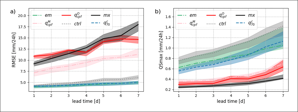
The best forecast as measured by a given performance measure can be the worst forecast with another performance metric. Verification results of precipitation point-forecasts in terms of (a) root mean squared error (RMSE) and (b) quantile score for a probability level of 98% (QSmax) as a function of the forecast lead time. For both performance metrics, the lower the better. The different types of forecasts are discussed in the text.
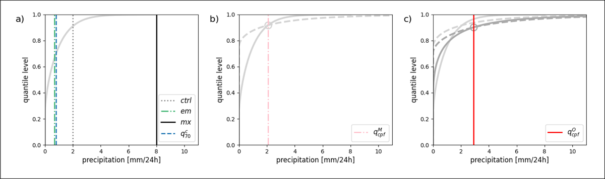
Figure 2
Types of point-forecasts investigated in this study as illustrated with a synthetic example: (a) a deterministic forecast (ctrl), a forecast ensemble distribution (solid gray line) with the corresponding ensemble mean (em), ensemble maximum (mx) and conditional 70% quantile (); (b) the model climate (dashed gray line), the intersection point with the ensemble distribution, and the corresponding self-adaptive quantile (); and (c) same as (b) but when considering the observation climate and a calibrated ensemble (dark gray) to define the self-adaptive quantile ().
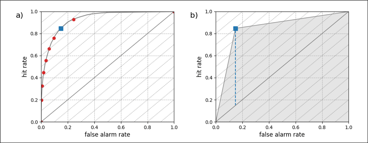
Figure 3
(a) Relative operating characteristic (ROC) curve for a probability forecast where each point corresponds to results for a different probability threshold. The blue square corresponds to the probability threshold that maximizes the Peirce skill score (PSS). (b) Area under the ROC curve for the optimal probability threshold is shown in gray while the corresponding PSS is indicated by a blue dashed vertical line.
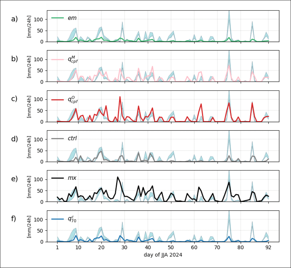
Figure 4
Time series of point-forecasts with corresponding observation over summer 2024. The maximum precipitation over a 10×10 grid-point area centered over Toulouse, France, is shown. The day indicated on the x-axis corresponds to the forecast starting date. All forecasts have a lead time of 5 days: (a) ensemble mean em, (b) adaptive-quantile with model climate , (c) adaptive-quantile with radar climate , (d) control member ctrl, (e) maximum of all ensemble members mx, and (f) conditional 70%-quantile . On each plot, the radar observation is represented by two dashed curves corresponding to the mean and maximum value within the area.
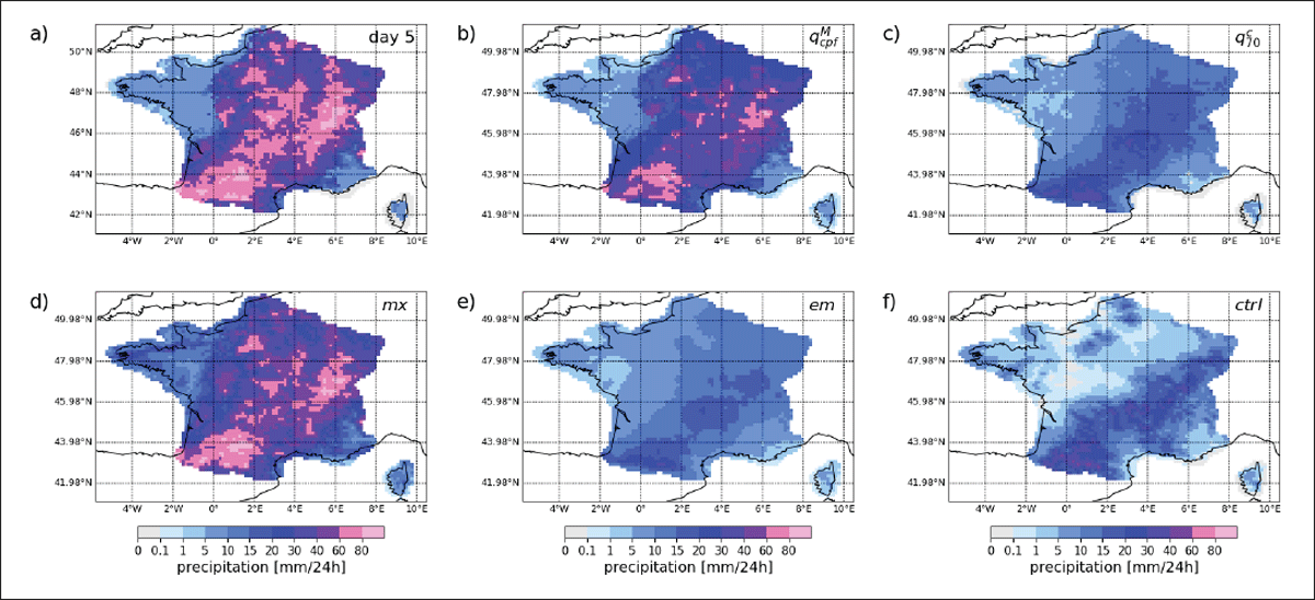
Figure 5
Point-forecasts at day 5 valid on August 14, 2024: (a) crossing-point quantile based on the radar climatology, (b) crossing-point quantile based on the model climatology, (c) conditional 70%-quantile forecast, (d) maximum of all ensemble members, (e) ensemble mean, and (f) control forecast.
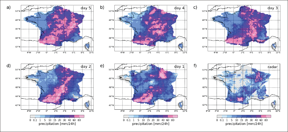
Figure 6
Crossing-point quantile forecasts for consecutive runs (a) to (e), all valid on August 14, 2024, and (f) the corresponding radar observation.
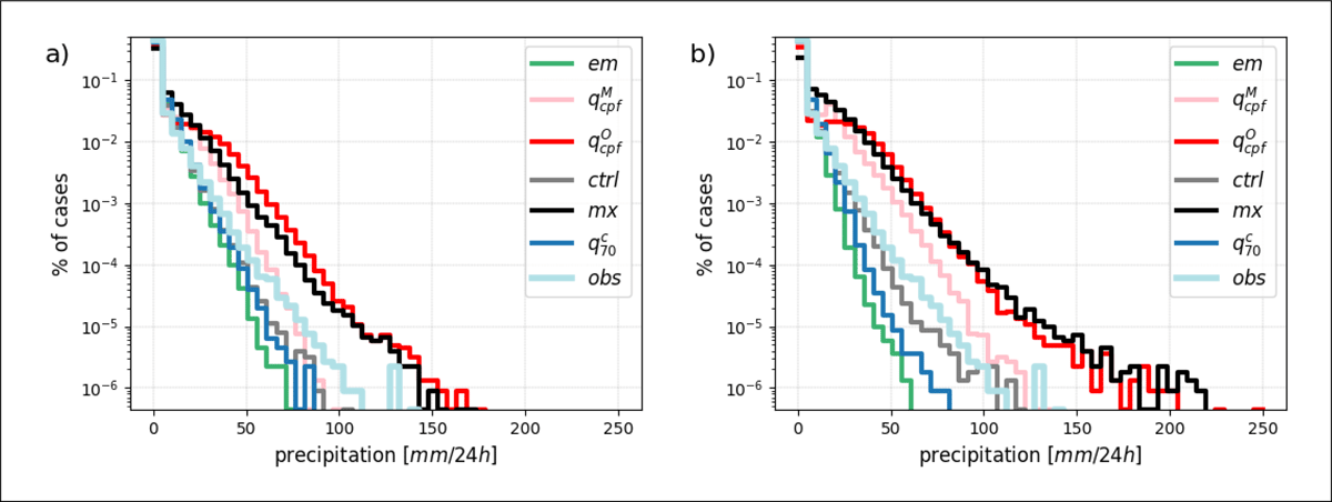
Figure 7
Observation and point-forecasts distributions at (a) day 1 and (b) day 5.
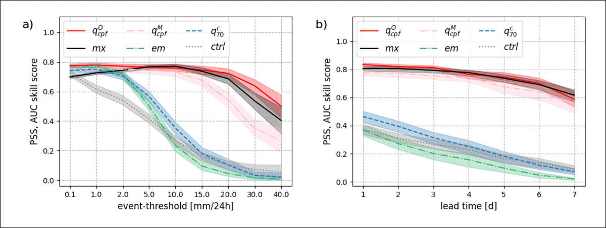
Figure 8
Peirce skill score (PSS) or equivalently area under the relative operating characteristic (ROC) curve (AUC) skill score (a) as a function of the event threshold for a lead time of 5 days and (b) as a function of the lead time for an event threshold of 15 mm/24 h.
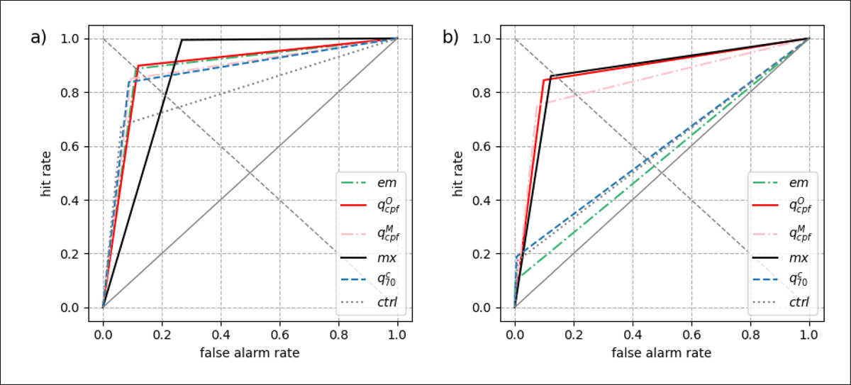
Figure 9
Relative operating characteristic (ROC) curves at day 5 for an event threshold of (a) 1 mm/24 h and (b) 15 mm/24 h.
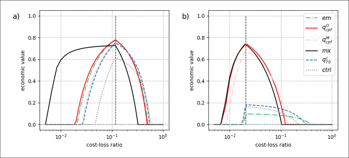
Figure 10
Same as Figure 9 but for the economic value.