
1 Introduction
While weather forecasting was approached as a deterministic initial value problem at the beginning of the 20th century (Bjerknes, 1904), ensemble prediction systems are nowadays common practice in meteorology and many other scientific fields (Chen, 2024). Ensembles consist of a set of plausible weather outcomes that allow the uncertainty about the future state of the atmosphere to be estimated (Leith, 1974). Accounting for forecast uncertainty in decision-making has proven more valuable than relying on a single best-guess forecast (Cooke, 1906; Roulston and Smith, 2004, and others in between).
Forecast end-users’ ability to deal with uncertainty is, however, heterogeneous. For some end-users, the uncertainty associated with a forecast is useful (Joslyn and Savelli, 2010; Morss et al., 2008), while for others, this information is difficult to apprehend (Fundel et al., 2019). Strategies to account for forecast uncertainty can consist in extracting a summary forecast that would, in the long term, optimize one’s decision-making process.
Moreover, automation of forecasting tasks are developed by meteorological agencies to mitigate production overload and limited resources (Pagano et al., 2016). By nature, forecast automation relies on maximizing a measure of accuracy. In this context, the question arises of how the diversity of information generated by an ensemble, on the one hand, and the automation requirement, on the other hand, can fit together while acknowledging the diversity of users’ needs. One approach is to derive a single actionable forecast potentially suitable for a wide range of users.
So-called best-guess forecasts can be derived from an ensemble by using, for example, clustering. Different clustering techniques exist to create consistent scenarios, with one single model representing a cluster (Ono, 2023). However, the use of a single model is questionable: the definition of the best member is a highly multidimensional task (Roulston and Smith, 2003), and the concept of the dominance of one model among all realizations is sometimes considered a flawed concept (Bright and Nutter, 2004).
Alternatively, the whole ensemble can be used to create a pseudo-deterministic meteorological field, the so-called consensus forecast (Roebber, 2010). For example, optimal forecast with respect to square and/or absolute errors can be derived using genetic programming (Bakhshaii and Stull, 2009) or spatially patched precipitation field from ensemble members closest to the mean (Schwartz et al., 2014). More recently, optimal threshold optimization based on F2 and Equitable Threat Score has been empirically investigated by Bouttier and Marchal (2024). A common aspect of all these studies on consensus forecasts is that optimization relies on the definition of a measure of accuracy.
What is the ideal consensus forecast for a given measure of accuracy? The answer to this question is related to the concept of forecast elicitation or consistency with a scoring rule (Ziegel, 2016). The development of a mathematical framework for a formal definition of elicitation is out of scope here, but we introduce this concept based on two simple examples: (1) the ensemble mean is consistent with the root mean squared error (RMSE) and (2) quantile forecasts are consistent with quantile scores (QS). A special case of the latter is the 50% quantile (or median), which is consistent with the mean absolute error.
Figure 1 illustrates the concept of elicitation with two examples. While more details about the data and the different forecast types are provided below, we can make the following remarks. The ensemble mean (em) is the best-performing forecast in terms of RMSE for all lead times in Figure 1(a). The concept of elicitation is powerful because one does not need to test if the ensemble mean is the best forecast in terms of RMSE for a given application, but rather should know beforehand that it is the case. Similarly, the quantile forecast (mx) is the best forecast in terms of the quantile score QSmax for all lead times in Figure 1(b), as expected. In this example, em is one of the worst performing forecasts in terms of QSmax, and mx is the worst performing forecast in terms of RMSE. In other words, the best forecast for one application can be the worst for the other one.
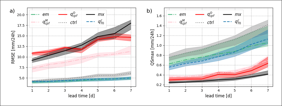
Figure 1
The best forecast as measured by a given performance measure can be the worst forecast with another performance metric. Verification results of precipitation point-forecasts in terms of (a) root mean squared error (RMSE) and (b) quantile score for a probability level of 98% (QSmax) as a function of the forecast lead time. For both performance metrics, the lower the better. The different types of forecasts are discussed in the text.
In this manuscript, we introduce a new type of point-forecast, the crossing-point quantile, and demonstrate that this forecast is optimal in terms of Peirce skill score (PSS, Peirce, 1884) in case of a reliable ensemble system, whatever the event of interest. The work presented here is based on the crossing-point forecast (CPF) developed and explored in previous studies. Ben Bouallègue (2021) showed that the CPF is consistent with the Diagonal score, a threshold/quantile-weighted continuous ranked probability score introduced in Ben Bouallègue et al. (2018).
This paper is organized as follows: Section 2 introduces the point-forecasts used for comparison together with a description of the theoretical properties of the crossing-point quantile. Section 3 displays illustrations of forecasts and observations alongside an analysis of the consistency between them. Section 4 discusses verification results before concluding in Section 5.
2 From ensemble to point-forecasts
2.1 Benchmarking
We start with the ensemble prediction system run at the European Centre for Medium-Range Weather Forecasts (ECMWF). The control member and the 50 perturbed ensemble members serve as a basis for deriving point-forecasts. A point-forecast is defined as a single-valued forecast expressed in the unit of the weather variable of interest. A deterministic forecast for temperature at, say, Reading, UK, tomorrow is a point-forecast. Another example is the ensemble mean for the same quantity.
In this study, we propose to compare the performance and characteristics of different point-forecasts with a focus on daily precipitation and time ranges up to the medium range. As a benchmark, we consider the following point-forecasts:
a deterministic forecast, here the ensemble control member (ctrl),
the ensemble mean (em), which is typically a smoothed field at longer time ranges as predictability decreases,
the maximum of all ensemble members (mx), which can also be interpreted as a quantile forecast at probability level with M the ensemble size1,
the quantile at a probability level of 70% conditioned on that at least half of the ensemble members indicates rain (). This latter is the consensus forecast used at Météo-France as a medium-range precipitation forecast.
These four types of point-forecasts are illustrated with a synthetic example in Figure 2(a).
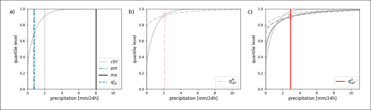
Figure 2
Types of point-forecasts investigated in this study as illustrated with a synthetic example: (a) a deterministic forecast (ctrl), a forecast ensemble distribution (solid gray line) with the corresponding ensemble mean (em), ensemble maximum (mx) and conditional 70% quantile (); (b) the model climate (dashed gray line), the intersection point with the ensemble distribution, and the corresponding self-adaptive quantile (); and (c) same as (b) but when considering the observation climate and a calibrated ensemble (dark gray) to define the self-adaptive quantile ().
2.2 Self-adaptive quantiles
Let us now remind the reader of the definition of the crossing-point forecast. For this, consider a condition called single intersection condition. Denoting as F and G as two cumulative distribution functions, F and G satisfy the single intersection condition if there is one unique q such that:
and
In this situation, the intersection between F and G is defined by the point (q,F(q)). If F is a forecast and G a climatology, F(q) is the so-called crossing-point forecast (Ben Bouallègue, 2021). By analogy, q is called the crossing-point quantile, which is the focus of this study.
The concept of crossing-point forecast and quantile is illustrated in Figure 2(b). The single intersection point between the ensemble distribution (F, represented by a solid gray line) and the climatology distribution (G, represented by a dashed gray line) is indicated by a circle. CPF is the projection of this point on the y-axis and so takes a value between 0 and 1 (not shown). In other words, CPF is a quantile level that varies for each forecast. Consequently, the crossing-point quantile q is a self-adaptive-quantile forecast, a quantile forecast at a quantile level corresponding to the CPF of the day (indicated by a pink vertical line).
In the estimation of the CPF, forecast and climate distributions refer to the same space, the “model space.” In that case, the crossing-point quantile is denoted by as it is based on the model climate. When issuing an adaptive-quantile forecast, one can consider using an observation climatology instead of a model climatology. To be consistent and to ensure forecast reliability, the ensemble can be calibrated in the “observation space.” The calibrated forecast and observation climatology can differ from the raw forecast and the model climatology, respectively, as illustrated in Figure 2(c). When based on a calibrated forecast and the observation climatology, the crossing-point quantile is denoted by .
More details about how model and observation climate distributions are built in our experiments can be found in Appendix A while a short description of the methodology followed to calibrate the ensemble is provided in Appendix B.
2.3 The optimal forecast in terms of PSS
The Peirce skill score (PSS) is a verification metric for dichotomous (yes/no) forecasts assessed against dichotomous observations (an event happens or not). We can show that the crossing-point quantile forecast is the optimal forecast in terms of PSS for any event.
Let us first define PSS. Consider a dichotomous forecast for a yes/no event (typically the observation being greater than a threshold). For verification, a contingency table is populated by counting the number of hits (A), false alarms (B), misses (C), and correct negatives (D). The hit rate (HR) is defined as the ratio while the false alarm rate (FAR) is defined as the ratio . The PSS definition is as follows:
A direct link exists between PSS and the relative operating characteristic (ROC) curve. For a dichotomous forecast, the ROC is defined by the point [FAR, HR]. In that case, Manzato (2006) showed that PSS and the area under the ROC curve (AUC) are related as follows:
The right-hand side of Eq. (4) is also known as the ROC skill score.
Now, consider a forecast for a binary event that takes the form of a probability. In that case, the ROC curve is a set of points [FAR, HR] estimated for a range of probability thresholds. A theoretical ROC curve for a probability forecast is illustrated in Figure 3(a). In this situation, the point closer to the left top corner of the plot corresponds to the probability threshold that maximizes PSS (i.e., the difference between HR and FAR). If the forecast is reliable, it can be shown that the tangent to the ROC curve at that point has a slope equal to 1 and that this point corresponds to the results obtained with a probability threshold equal to the event base rate (Ben Bouallègue et al., 2015; Richardson, 2011). This latter characteristics (the optimal probability threshold is equal to the event base rate) is key in the following demonstration.
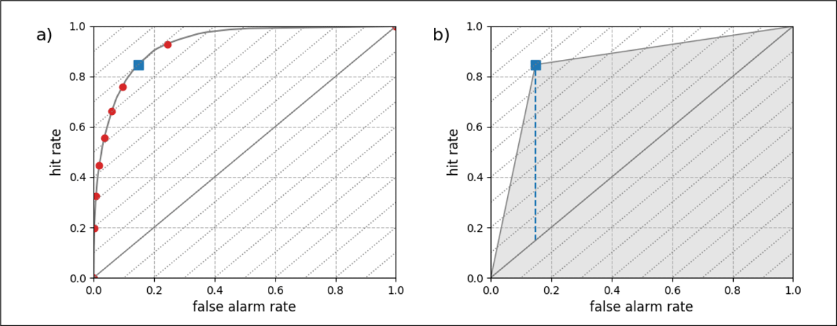
Figure 3
(a) Relative operating characteristic (ROC) curve for a probability forecast where each point corresponds to results for a different probability threshold. The blue square corresponds to the probability threshold that maximizes the Peirce skill score (PSS). (b) Area under the ROC curve for the optimal probability threshold is shown in gray while the corresponding PSS is indicated by a blue dashed vertical line.
Now, coming back to the crossing-point forecast, let us define more formally an event of interest, say x>θ with θ the event threshold (e.g., rain observed greater than 15 mm/24 h). The base rate of this event, denoted by pc, is by definition equal to 1–G(θ), where G is the climate cumulated probability distribution. We denote pf as the probability forecast for this event, which is by definition 1–F(θ), where F is the forecast cumulated probability distribution. Using Eqs (1) and (2), we can derive the following:
and
In plain words, Eqs (5) and (6) mean that taking action when the probability forecast pf is greater than the event base rate pc is equivalent to taking action when the crossing-point quantile q exceeds the event threshold θ. The former corresponds to the optimal choice to maximize PSS. So, conditioned on reliability, the crossing-point quantile is the optimal forecast in terms of PSS (and equivalently in terms of ROC area) for any dichotomous event defined by a threshold.
3 A qualitative assessment
We now assess qualitatively the different types of point-forecasts using case studies. For this purpose, we show two types of plots: (1) time series of precipitation maxima within an area over consecutive summer days and (2) maps of precipitation fields for an interesting date in the series.
The observation used to compute statistics, build a climatology, and illustrate this article is a radar dataset called COMEPHORE (COmbination for Best Estimation of Hourly Precipitation). This hourly precipitation reanalysis product is based on radar and rain gauge data, covering metropolitan France (Tabary et al., 2012).
The data, originally on a 1 km grid, are aggregated at the spatial resolution of the ensemble forecast, that is, 18 km. The upscaling of the observation consists in averaging the precipitation at the new spatial scale. This step is applied consistently in the verification and in the observation climatology. This choice aims at a fair comparison of the different point-forecasts evaluated here, all interpreted as averaged precipitation over a grid box. For operational purposes, one could instead consider using a COMEPHORE climatology at the original scale to benefit from a downscaling while estimating the crossing-point quantile.
3.1 Time series
We define an area of 10×10 model grid points centered over Toulouse, France. For each forecast as well as for the radar, the maximum precipitation within this area for each day is shown in Figure 4. The time series cover June, July, and August (JJA) 2022.
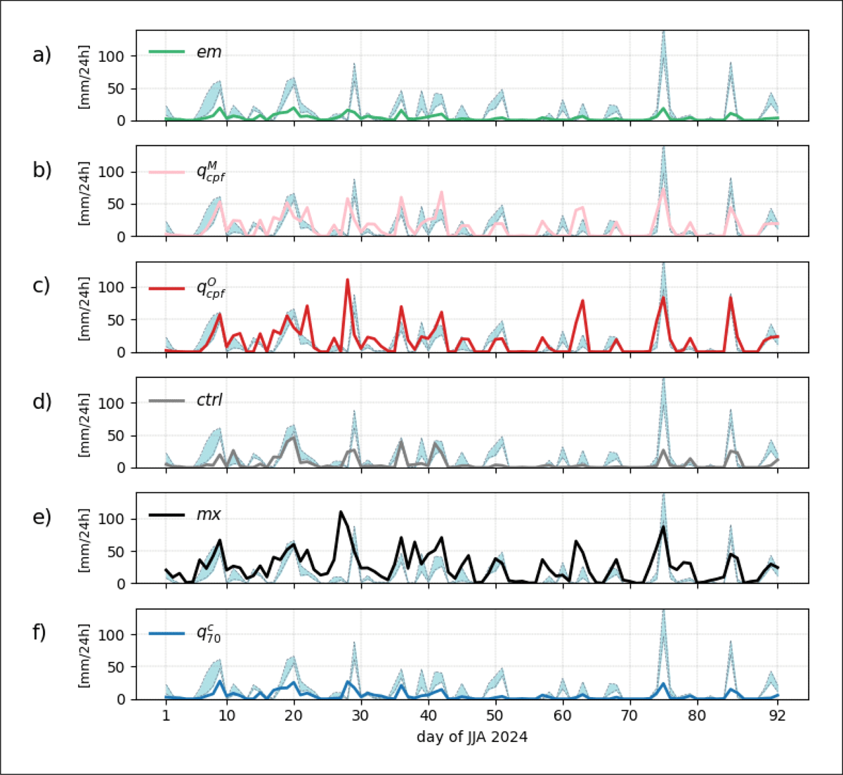
Figure 4
Time series of point-forecasts with corresponding observation over summer 2024. The maximum precipitation over a 10×10 grid-point area centered over Toulouse, France, is shown. The day indicated on the x-axis corresponds to the forecast starting date. All forecasts have a lead time of 5 days: (a) ensemble mean em, (b) adaptive-quantile with model climate , (c) adaptive-quantile with radar climate , (d) control member ctrl, (e) maximum of all ensemble members mx, and (f) conditional 70%-quantile . On each plot, the radar observation is represented by two dashed curves corresponding to the mean and maximum value within the area.
The ensemble mean (em) systematically underestimates the precipitation amount, but larger em values (in relative terms) are generally associated with larger observations. The crossing-point quantiles, both and , show a good fit with the observations, with the former () displaying larger values that match better with the observations in this example. With the control member (ctrl), several large precipitation events are missed while the ensemble maximum (mx) is more prone to false alarms with sometimes large forecast values when no rain is observed. Finally, the conditional quantile () shows a systematic underestimation of large precipitation events.
The most extreme precipitation event observed in the series was on August 14 (day 75). This event seems particularly well captured by the crossing-point quantiles with an intensity closer to the observation for . We now assess visually the forecasts as fields valid on that particular date.
3.2 Maps
The case study discussed here refers to August 14, 2024, identified as the most extreme event during the summer of 2024 in the Toulouse area. The different point-forecasts are shown in Figures 5(a) to 5(f), all have a forecast lead time of 5 days. In Figures 6(a) to 6(e), we focus on the crossing-point quantile forecasts and compare forecasts at decreasing lead times but with the same validity time.
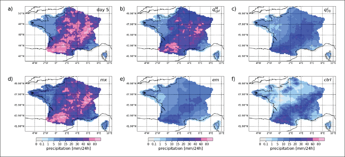
Figure 5
Point-forecasts at day 5 valid on August 14, 2024: (a) crossing-point quantile based on the radar climatology, (b) crossing-point quantile based on the model climatology, (c) conditional 70%-quantile forecast, (d) maximum of all ensemble members, (e) ensemble mean, and (f) control forecast.
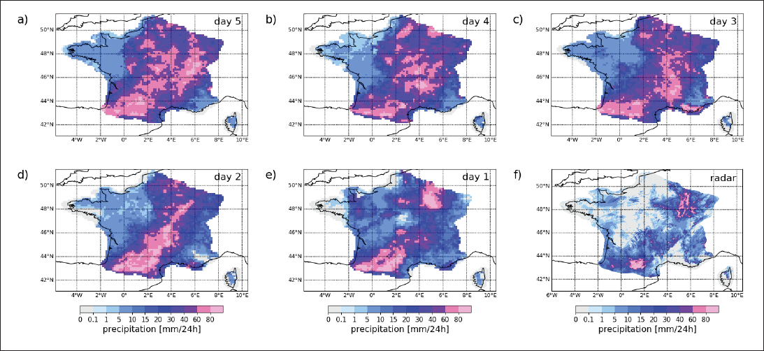
Figure 6
Crossing-point quantile forecasts for consecutive runs (a) to (e), all valid on August 14, 2024, and (f) the corresponding radar observation.
The radar observation for the verification date is shown at its native resolution in Figure 6(f). The radar captured the strongest precipitation signal over the South West of France with values exceeding 80 mm/24 h. High precipitation values are also registered along a South-West/North-East axis with larger scale precipitation in the North-East of France.
In this example, the crossing-point quantiles shown in Figures 5(a) and 5(b) exhibit heavy precipitation forecasts over the whole of France except Brittany and the South-East, with larger values in . In Figure 5(c), the conditional quantile shows a similar picture but with an intensity typically twice smaller than . As shown in Figure 5(d), the maximum of all members forecast more than 5 mm/24 h of rain over the whole country with large value (greater than 40 mm/24 h) all along a South-West/North-East axis. As shown in Figures 5(e) and 5(f), the ensemble mean and control forecast, respectively, performed poorly at this lead time with generally lower precipitation rates than in the radar and missed events in the North-East.
Figures 6(a) to 6(e) shows the evolution of a crossing-point quantile forecast over consecutive runs. Typically, the adaptive-quantile forecast would indicate larger areas with potentially extreme events at longer lead times (when the forecast uncertainty is large). As we approach the time of the event, the forecast is sharper with smaller areas indicating the potential occurrence of an extreme event. The forecast also appears less noisy at shorter lead times. More ensemble members would allow better capturing the tail of the forecast distribution and thus help reduce the forecast noise in the medium range.
3.3 Forecast consistency
Is one type of forecast generally overestimating or underestimating the observed precipitation? The examples shown in Figures 4 and 5 seem to indicate that this is the case but to answer this question systematically, we compare the distributions of the forecast and the observation. Here, we define equally spaced bins and count the number of cases falling in each bin over the verification period. The results are shown in Figure 7.
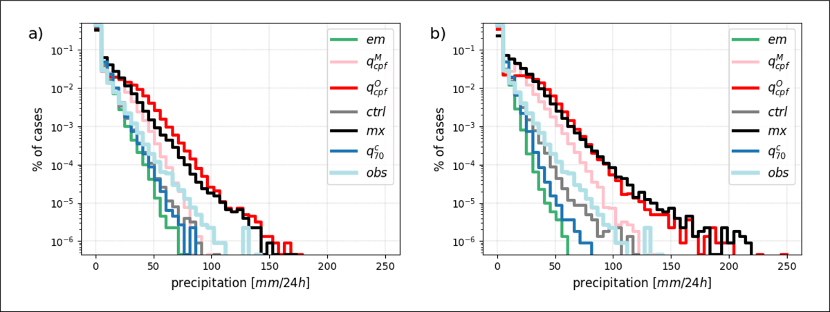
Figure 7
Observation and point-forecasts distributions at (a) day 1 and (b) day 5.
In Figure 7(a), the forecast distributions at day 1 generally resemble the observation distribution with two striking exceptions: the ensemble mean (em) tends to systematically underestimate the highest precipitation while the maximum of all ensemble members (mx) tends to systematically overestimate it. It is worth noting that the control forecast (ctrl) shows good consistency with the observations. Here, the control forecast is the only point-forecast that is also a coherent scenario (in space and time).
As a consequence, at day 5, as shown in Figure 7(b), the control forecast is the only forecast that still has some resemblance with the observation in terms of distribution. The other point-forecast distributions are somehow modulated by the uncertainty in the forecast at that time range. Ensemble mean (em) and conditional quantile () show a clear underestimation of larger precipitation values while the ensemble maximum tends to underestimate low precipitation amounts. Focusing on the tail of the observation distribution, we note that only the self-adaptive quantiles and the maximum of all members are able to generate the highest amount of precipitation observed in the radar (above 100 mm/24 h).
4 A quantitative assessment
A quantitative assessment complements the qualitative comparison based on case studies and the consistency check presented in Section 3. In this section, we discuss averaged scores computed for three consecutive summers, that is June, July, and August in 2022, 2023, and 2024.
4.1 Optimal point-forecasts
The first result was already presented in Figure 1: the ensemble mean is the best forecast in terms of RMSE (Figure 1a) while the ensemble maximum is the best forecast in terms of QSmax (Figure 1b). The crossing-point quantile forecasts and are “intermediate” forecasts for both metrics with a larger variability in leading to worse RMSE performance.
In theory, the crossing-point forecast should be the optimal forecast in terms of PSS for any event as discussed in Section 2.3. Whether this property holds in practice is explored in Figure 8. The PSS (equivalently the AUC) are shown for a range of event thresholds from 0.1 mm/24 h up to 40 mm/24 h and for a range of forecast lead times from day 1 to day 7. Figure 8(a) focuses on one lead time (day 5) while Figure 8(b) focuses on one event threshold (15 mm/24 h).
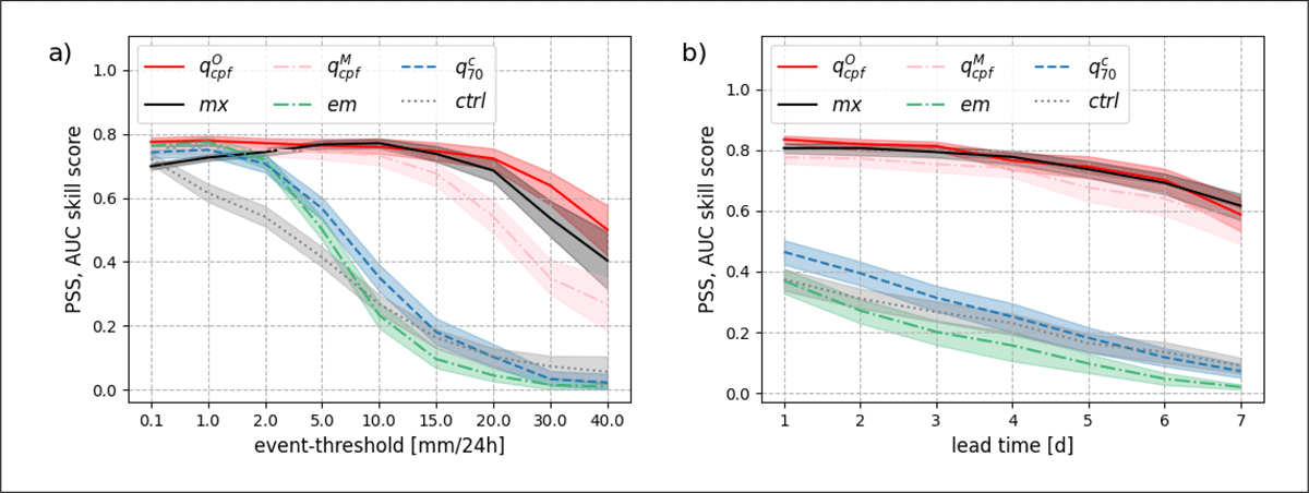
Figure 8
Peirce skill score (PSS) or equivalently area under the relative operating characteristic (ROC) curve (AUC) skill score (a) as a function of the event threshold for a lead time of 5 days and (b) as a function of the lead time for an event threshold of 15 mm/24 h.
Figure 8 supports our theoretical findings: the crossing-point forecast is the best or among the best forecasts compared here in terms of PSS (within score uncertainty margins). This result holds for all lead times. Importantly, we note that calibration plays a key role to reach this level of skill: calibration is a necessary condition for optimality.
Focusing on day 5, Figure 9 shows ROC curves for two events: precipitation exceeding 1 mm/24 h and 15 mm/24 h in Figure 9(a) and 9(b), respectively. Typically, the ensemble maximum has a higher false alarm rate than optimal for smaller thresholds while the ensemble mean and control forecast tends to have a smaller hit rate than optimal for higher thresholds. Also, the impact of calibration is visible in Figure 9(b) with a ROC point for closer to the top-left corner of the plot than : calibration is needed to ensure optimality for higher event thresholds.
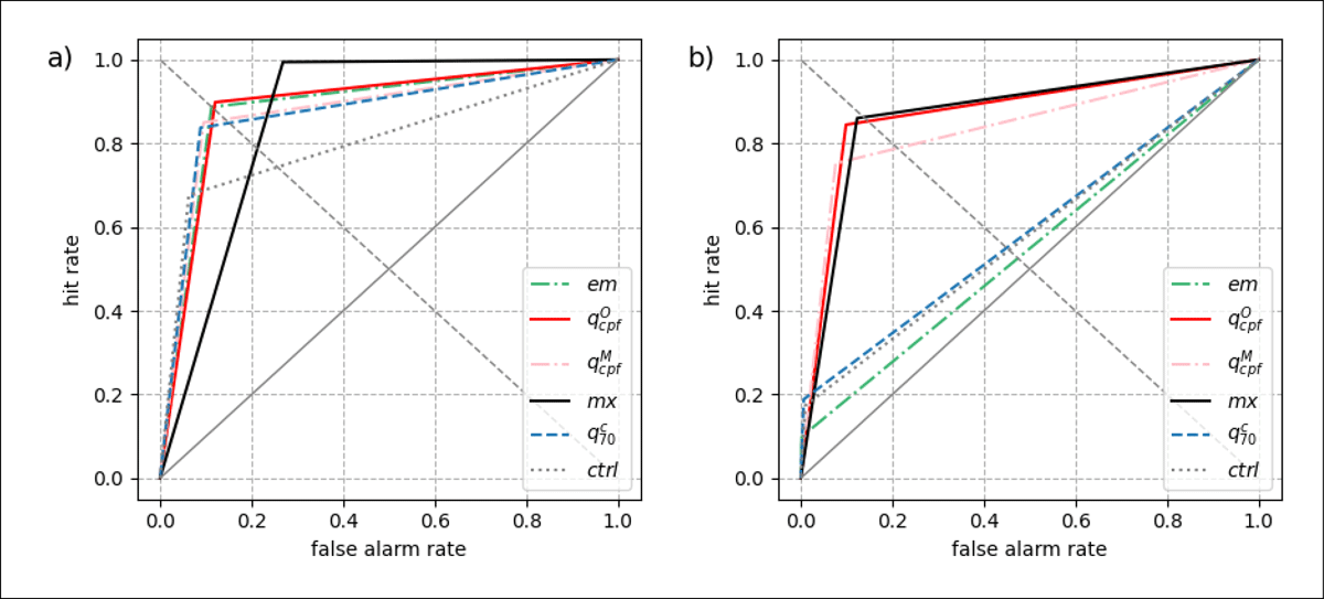
Figure 9
Relative operating characteristic (ROC) curves at day 5 for an event threshold of (a) 1 mm/24 h and (b) 15 mm/24 h.
4.2 Economic value
The economic value of a forecast is estimated here with the help of a simple cost-loss model. We consider the case where a forecast user can mitigate the loss associated with the occurrence of a weather event by taking a preventive action. The user decides to take action or not based on the forecast. The key parameters of this model are (1) the cost of taking action and (2) the loss encountered if no protective action is taken but the event occurs. The cost-loss ratio characterizes the user in the sense that it reflects a specific user-defined application. Building on this model, the so-called potential economic value is derived from the elements of the contingency table (Richardson, 2000).
Figure 10 compares the economic value of different types of point-forecasts as a function of the user’s cost-loss ratio. Figures 10(a) and 10(b) focus on two different events defined as precipitation exceeding 1 mm/24 h and 15 mm/24 h, respectively. Both plots are results for forecasts at a lead time of 5 days. Note that a logarithmic scale is used for the x-axis in Figure 10 that put more emphasis on low cost-loss ratios. The ensemble maximum has a higher economic value for very low cost-ratios, and adaptive-quantile forecast has a higher economic value than other forecasts for cost-loss ratios in the range of the event base-rate (indicated by a vertical line). For applications with larger cost-loss ratios, the conditional quantile and ensemble mean are better choices for decision-making.
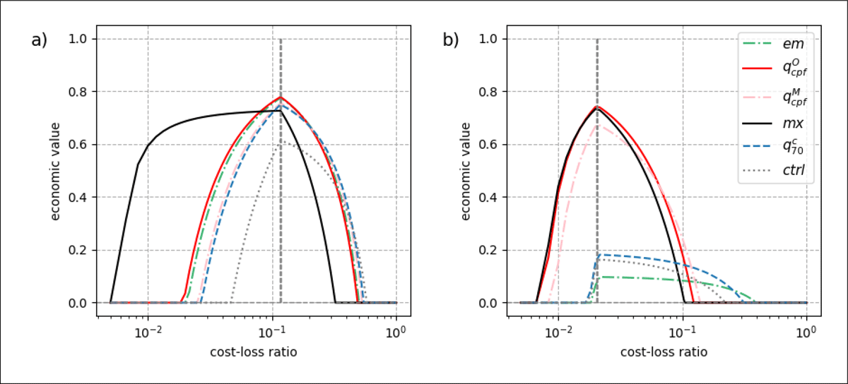
Figure 10
Same as Figure 9 but for the economic value.
5 Summary and outlook
The crossing-point is the intersection point between two cumulative probability distributions: a forecast and a climatology. The corresponding quantile varies with the forecast uncertainty of the day. This self-adaptive-quantile forecast is called the crossing-point quantile forecast. In our study, we discussed the properties and performance of this new type of point-forecast. Our summary points and outlook are as follows:
Elicitation. The link between crossing-point forecast and PSS is similar to the link between mean forecast and RMSE, or median forecast and MAE. Indeed, we demonstrate that the crossing-point quantile is the optimal forecast in terms of PSS (and equivalently in terms of ROC area) for any event. Furthermore, the crossing-point quantile links the PSS with the Diagonal score, which can be interpreted as a weighted average of AUC, as shown in Appendix C.
Extreme events. Optimality for any event includes optimality for rare and extreme events. We showcase the crossing-point performance with case studies and statistical analysis that support our theoretical findings. The predictive power of the crossing-point forecast for extreme events is also explored in Ben Bouallègue (2024).
Condition of optimality. The necessary condition for optimality is calibration. The ensemble or probabilistic forecast needs to be well-calibrated to ensure a theoretical guarantee of optimality. When necessary, statistical post-processing can be applied to reach that goal (Vannitsem et al., 2021).
Model climate. When post-processing is used to calibrate the forecast, there is no need to build an M-climate based on reforecasts (which can be expensive). After calibration in the observation space, the climate distribution used to build the CPF would be directly estimated from observations for consistency. In the case of a well-calibrated system, model and observation have the same climatology.
Observation climatology. The estimation of climate percentiles can be a moving target due to natural variability and anthropogenic climate change. When one build a climatology with limited observation records, one could consider using extreme value theory to better capture the tail of the distribution. For example, non-negative precipitation amounts can be fitted with an Extended Pareto Distribution as suggested by Naveau et al. (2016).
Interpretation. Like any other quantile forecast, a self-adaptive-quantile forecast based on the CPF is not a physically consistent spatial or temporal scenario. A crossing-point quantile forecast should be interpreted at each location (grid-point) as a local “probabilistic worst-case scenario” (Ben Bouallègue, 2021). In simple terms, the users are dealing with a state-dependent quantile, where the quantile level becomes more extreme as the predicted probability of an extreme event increases, a situation already observed in practical cases (Schmidt et al., 2021).
Usage. Self-adaptive-quantile forecasts are particularly well-suited for users whose cost-loss ratio is unfocused, that is, with a cost-loss ratio that decreases as the rarity of the event increases. As revealed by our economic value analysis, the crossing-point quantile forecast is not suitable for all users. In particular, users sensitive to false alarms might consider using the ensemble mean instead, which displays large values only when the forecast uncertainty is small.
Loss function. In principle, weighted proper scores could be used as loss functions to train weather forecasting models based on machine learning. For example, one could consider the Diagonal score which is consistent with the crossing-point forecast as a performance metric. The link between Diagonal score, PSS, and the coefficient of predictive ability (CPA, Gneiting and Walz, 2022) is developed in Appendix C.
Outlook. The quality of the CPF predominantly depends on the quality of the underlying ensemble prediction system. So, improvement for this new type of prediction would lie in (1) better raw (or post-processed) ensemble forecasts and (2) more ensemble members for a finer estimation of the intersection point between distributions. Machine learning could help achieve these objectives in a near future.
Appendix
A Model and radar climatology
The model climatology, also known as M-climate, is built on 20 years of reforecasts. A period of 5 weeks centered around the current day is used to account for seasonal variations as described in Lalaurette (2003). Similarly, an observation climatology is estimated for each week of the year using a 5-week rolling period over 20 years of records from 2001 to 2020.
B Ensemble calibration
Ensemble calibration is based on a member-by-member approach (MBM, Van Schaeybroeck and Vannitsem, 2015) and tested successfully on ensemble precipitation forecasts (e.g., Ben Bouall‘egue et al., 2024). A correction is applied to each ensemble member individually with a component common to all members and a component that adjusts the deviation of a member with respect to the ensemble mean. If we denote the corrected forecast for the mth member of the ensemble, MBM formally consists in applying:
where xi is the ensemble member i and is the ensemble mean. A clipping to zero is applied to the corrected forecast. The parameter α is the bias parameter that nudges the ensemble mean, β is the linear coefficient that scales the ensemble mean, and γ is the scaling parameter that adjusts the spread of the ensemble. The coefficients α, β, and γ are estimated over the summer of 2021 for all grid points together but for each forecast lead time independently.
C Diagonal score, Peirce skill score, and universal ROC
Following Ben Bouallègue (2021), the Diagonal score DG is defined using elementary scores dG as follows:
with G the climatology probability distribution, F the forecast probability distribution, and
When the observation ranges the unconditional distribution G, the expectation of the elementary Diagonal score is a function of PSS:
with and , respectively the hit rate and the false alarm rate associated to the event G–1(1–α). For the climatological forecast, .
In this framework, PSS can be written as the elementary diagonal skill score:
Similarly, the expected Diagonal score can be understood as a sum of quadratic weighted PSS:
Thus the expected Diagonal score of a climate forecast G is 1/6. This score is obtained for any non-informative forecast, that is, a forecast for which Hα=Fα. In other words, the Diagonal score is equitable.
Moreover, Gneiting and Walz (2022) defined the CPA as a general measure of potential predictive ability. CPA takes value between 1/2 and 1 and is equivalent to the area under the universal ROC, obtained by convex combinations of ROC curves for any event of interest. In the case of point-forecasts, the CPA can be informally defined as follows, up to a multiplicative factor:
As a result, the general measure of predictive ability of Gneiting and Walz (2022) is equivalent to the Diagonal skill score:
The crossing-point quantile is also elicitable with respect to the same scoring function (the Diagonal score) as being a differentiable transformation of the crossing-point forecast. This result is derived from the work of Osband (1985), later recalled by Gneiting (2011) and Fissler and Ziegel (2016) among others.
Notes
[1] If one would like to optimize the continuous ranked probability score, the ensemble members must be interpreted as quantile forecasts at probability levels with according to Bröcker (2012).
Acknowledgements
The authors are grateful to an anonymous reviewer for their insightful and constructive comments. Also, MT would like to thank the University of Reading for hospitality and the Isaac Newton Institute for Mathematical Sciences for support during the satellite program “Geophysical fluid dynamics; from mathematical theory to operational prediction” when work on this paper was undertaken.
Competing Interests
The authors have no competing interests to declare.