
1 Introduction
In the modern ocean, the global ocean’s overturning circulation consists of two cells: an upper cell associated with the formation of North Atlantic Deep Water (NADW), and a lower cell associated with the formation of Antarctic Bottom Water (AABW) (Cessi, 2019; Marshall and Speer, 2012; Talley, 2013). In the top ~1000 m of the Atlantic basin, warm and salty surface waters overlying cold and fresh Antarctic Intermediate Water (AAIW) flow towards northern high latitudes, as shown in observations from the World Ocean Atlas 2018 (Boyer et al., 2018), along a meridional section along W in the Atlantic basin (Figure 1). In the northern high latitudes, surface buoyancy loss due to strong cooling leads to the transformation of the lighter limb of this meridional overturning circulation (MOC) to its denser limb, which then returns southwards between 1000 m and 3000 m depth (Figure 1). This upper overturning cell is known as the Atlantic MOC (AMOC).
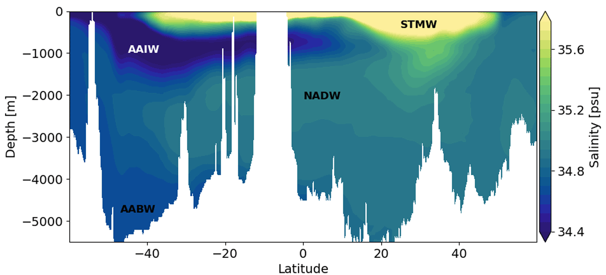
Figure 1
Realistic water mass structure. Salinities from the World Ocean Atlas 2018 along a meridional section at 37°W in the Atlantic basin. The main water masses are labelled as Antarctic Intermediate Water (AAIW), SubTropical Mode Water (STMW), North Atlantic Deep Water (NADW), and Antarctic Bottom Water (AABW).
In the southern hemisphere, adjacent to the Antarctic coast, surface buoyancy loss due to atmospheric cooling results in brine rejection during sea-ice growth and the formation of dense AABW. This formation of AABW forms the downward limb of the lower overturning cell which occupies the deepest part of the water column (Figure 1). This lower overturning cell is largely confined to the Pacific basin. A zonal integral of this overturning circulation across all ocean basins gives the well-known picture of a two-cell overturning circulation (Marshall and Speer, 2012). Despite its importance for global climate, there is still much controversy over what actually drives this overturning circulation, mainly as a result of different views on the role of convection in the ocean’s overturning circulation (Gayen and Griffiths, 2022; Hughes and Griffiths, 2008; Klocker et al., 2023a).
In the view dominant in the oceanographic literature, convection in high latitudes denotes a local process resulting from buoyancy loss due to surface forcing. In the open ocean this creates convective chimneys that stabilise the water column by mixing water properties in the vertical (Marshall and Schott, 1999) with little vertical flux of actual mass (Send and Marshall, 1995). This convection is presumed to be vital for the downward mass transport associated with the overturning circulation, but the link between both local convection and net downward mass transport remains inconclusive (de Jong and de Steur, 2016).
Given the local nature of convection in this view, the closure of the overturning circulation requires other processes that lead to the upward movement of these waters (Munk and Wunsch, 1998; Wunsch and Ferrari, 2004). While the theories on the upward component of the overturning have evolved over time, they all agree that the closure of the overturning circulation requires mechanical forcing by winds and/or tides (Munk and Wunsch, 1998; Wunsch and Ferrari, 2004), whether through Ekman pumping in the Southern Ocean (Marshall and Speer, 2012; Toggweiler and Samuels, 1995, 1998) or through vertical mixing in the ocean interior (Munk, 1966; Munk and Wunsch, 1998). In the former, the horizontal divergence of the wind forcing in the Southern Ocean leads to an upwelling from depth along density surfaces, and is crucial for the closure of the upper overturning cell. In the latter, the action of winds (and tides) leads to the generation of internal waves, which then dissipate into small-scale motion that causes vertical mixing.
In the absence of winds and tides, the overturning circulation (if viewed this way) would lead to a circulation confined to the ocean surface, with the deep ocean turning into a stagnant pool of cold water (Munk and Wunsch, 1998; Wunsch and Ferrari, 2004). If this were true, a “thermohaline” circulation, i.e. a circulation forced by only temperature and salinity at the ocean surface, would not lead to a full-depth overturning circulation as is observed in the ocean. This view of the overturning circulation leads to the question of what determines the vigour of the global ocean’s overturning circulation: the “push” of convection, leading to the formation of dense waters to depth in the polar regions, or the “pull” of mixing and Ekman transport bringing those waters upwards throughout the ocean basins (Visbeck, 2007).
The dominant view in the fluid dynamics literature is that, a full-depth overturning circulation can be generated by a flow configuration known as horizontal convection (Hughes and Griffiths, 2008; Stern, 1975). Horizontal convection is forced due to a lateral change in sign in surface buoyancy forcing, typically with buoyancy gain at low latitudes and buoyancy loss at high latitudes. As opposed to local convection which only requires buoyancy loss and hence a separate source of buoyancy gain, horizontal convection describes a full flow configuration in which the entire overturning circulation is solely driven by sources and sinks of buoyancy.
An example of horizontal convection in a laboratory experiment is shown in Figure 2. This forcing configuration, with heating on the top right and cooling on the top left, results in a horizontal flow from the heated to the cooled region. In the cooled part of the domain, the surface flow generates increasingly deeper convective cells until it reaches the endwall of the domain, leading to a full-depth vertical plume. This endwall plume is a region of full-depth convection and net downward mass transport. The horizontal surface flow produces a divergent velocity field, requiring an upward vertical velocity, which leads to a closure of the overturning loop through an advective-diffusive balance across the base of the planetary boundary layer (Gayen et al., 2014). A more detailed description of this process can be found in the review by Hughes and Griffiths (2008).
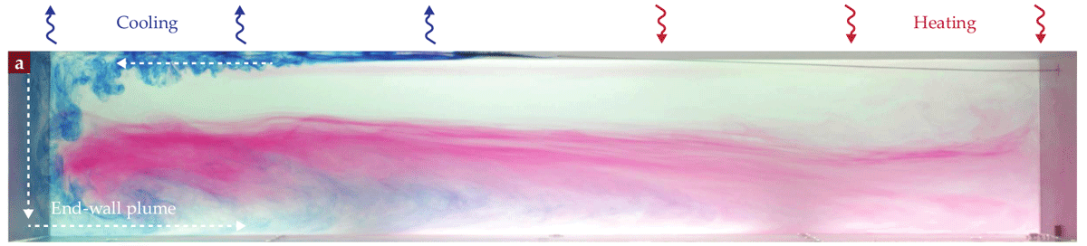
Figure 2
Horizontal convection. Horizontal convection is illustrated by the flow field from a laboratory experiment in a 3D rectangular box domain. The dye visualization shows the flow path from the heated region to the cooled region (right to left) along the upper boundary and broader bottom flow in the opposite direction. A full-depth end-wall plume is observed against the wall at the cooled end of the domain. Adapted from Gayen and Klocker (2024).
The reason that horizontal convection is not thought to be the relevant flow configuration to generate the ocean’s overturning circulation is that, despite generating a full-depth overturning circulation, stratification is confined to the surface of the fluid volume, with the majority of the interior volume being very weakly stratified. As a consequence, horizontal convection is not seen as being able to generate the mid-depth stratification observed in the ocean (Hazewinkel et al., 2012). This is why it has previously been thought that vertical diffusion is required to create this layer of enhanced stratification. As a consequence, assuming a priori that this mid-depth stratification is the consequence of an one-dimensional advection-diffusion balance, it has been estimated that a vertical diffusivity of is required to explain this stratification (Munk, 1966; Munk and Wunsch, 1998).
On the other hand, recent numerical experiments by Klocker et al. (2023a), simulating horizontal convection under a rotating environment in a range of idealised model domains, showed that this mid-depth stratification can also be generated in the limit of weak vertical diffusion. Here, the key to generating this mid-depth stratification in the presence of convection is the re-entrant channel domain, similar to the Southern Ocean (Barkan et al., 2013; Klocker et al., 2023a; Sohail et al., 2019). In such a domain, given the absence of meridional boundaries, a buoyancy gradient across the channel (such as that generated by convection along the southern boundary of the channel) leads to the steepening of isopycnal surfaces, and an associated circumpolar current, such as the Antarctic Circumpolar Current. These steep isopycnal surfaces then act to project the cross-channel surface buoyancy gradient along the sloping isopycnal surfaces onto the water column to the ocean basin(s) to the north, hereby stratifying the water column of the global ocean. Together with convection occurring at the northern boundary of the domain, this flow configuration results in a two-cell overturning circulation, separated by mid-depth stratification similar to that observed in the ocean (Klocker et al., 2023a).
Consistent with the understanding that flow in the ocean interior occurs along isopycnal surfaces, rather than across them, the mid-depth stratification required to close the overturning circulation is the consequence of an along-isopycnal, i.e. two-dimensional, advection-diffusion balance, as opposed to a vertical, i.e. one-dimensional, advection-diffusion balance, assumed by Munk (1966) and Munk and Wunsch (1998). Given that there cannot be any mean geostrophic transport across a re-entrant channel due to the absence of meridional boundaries, mesoscale eddies play a crucial role in closing the global ocean’s overturning circulation.
The experiments by Klocker et al. (2023a) had several caveats that made it difficult to assess this flow configuration’s role in explaining the global ocean overturning features and the resulting water mass distribution in the ocean. Two of these features we will improve on here, working step by step towards a more realistic simulation of the global ocean overturning circulation while learning what every step of complexity adds towards the realism of the simulations.
Firstly, we use both thermal and saline forcing and a nonlinear equation of state rather than the purely thermal forcing and linear equation of state used by Klocker et al. (2023a). Given the nonlinearities in the equation of state of seawater, salinity has a stronger control on the stratification in cold (polar) regions due to the large reduction of the coefficient of thermal expansion as a function of temperature. In contrast, at lower latitudes, stratification is controlled largely by temperature (Roquet et al., 2022). This explains why, for example, sea ice, through its effect on surface salinity, is the main control of high-latitude stratification (Klocker et al., 2023b). The nonlinear equation of state also leads to the processes cabbeling and thermobaricity, both important for the formation of AAIW and AABW (Groeskamp et al., 2016).
Secondly, we have added a second basin, a “Pacific” basin, to the single basin simulations of Klocker et al. (2023a). Several studies point out the potential importance of inter-basin exchanges in regulating the upwelling of deep waters (Jochum and Eden, 2015; Talley, 2013). However, these studies generally assume large rates of transformation of AABW into Deep Pacific Water to close the overturning circulation. However, recent studies have contended that the required mixing was leaving a Pacific shadow zone at mid-depth, essentially decoupling the bottom Pacific from the pycnocline (Holzer et al., 2021). Here, we will test how the coupling between lower and upper overturning cells is affected by the inclusion of a large basin with no active deep convection.
In Klocker et al. (2023a), the focus was on the processes generating the mid-depth stratification which could be achieved with a single basin and thermal forcing. Here we now focus on understanding if, and how, horizontal convection can generate the water mass structure observed in the ocean. In particular, we want to understand if horizontal convection forced by both temperature and salinity can generate the two-cell overturning structure and the resulting water masses, such as AAIW, NADW, and AABW, observed in the ocean. As mesoscale eddies play a crucial role in the dynamics of rotating horizontal convection in a re-entrant channel, we follow Klocker et al. (2023a) and use eddying model simulations. No wind forcing is applied to the model to understand how much of the circulation is explained by horizontal convection, without Ekman pumping by winds. Vertical diffusion is kept very low, limited by numerical diffusion, to approximate a limit in which winds and tides do not lead to vertical diffusion.
2 Model description
To investigate the role of thermal and haline forcing on the global ocean’s overturning circulation, we use the Massachusetts Institute of Technology general circulation model (MITgcm, Marshall et al. (1997)) in an idealised domain in spherical coordinates. This takes into account the full variation of the Coriolis parameter. The model configuration used here is based on that of Munday et al. (2013) and Klocker et al. (2023a). The horizontal model grid spacing is in the zonal direction, whereas the grid spacing in meridional direction is scaled by the cosine of latitude, making the grid boxes approximately square. The domain has a flat bottom with a depth of 5000 m, and hence no features such as, e.g. a ridge across Drake Passage. In the vertical, the domain is discretised by 42 unevenly spaced levels with a thickness of 10 m at the surface, increasing to 250 m at depth. We use a order advection scheme, no parameterisation for mesoscale eddies, both a harmonic and biharmonic Leith viscosity, and the vertical diffusivity for temperature and salinity in the reference case is set to . Convection is parameterised by an increased vertical diffusivity in case the water column becomes unstable. The nonlinear equation of state is that by Jackett and Mcdougall (1995). We run a total of ten experiments, as detailed in Table 1, varying a number of parameters as described below.
Table 1
Model experiments. “Basins” refers to either one narrow basin or two basins with a narrow basin representative of the Atlantic and a wide basin representative of the Pacific. “Salinity narrow basin” is the salinity that is being restored to at the northern boundary of either the single basin or the narrow basin in two-basin simulations. “Sea ice” refers to whether or not salinity at the surface is enhanced to psu adjacent to the southern boundary to simulate brine rejection. “Rotation” refers to either normal planetary rotation of Earth or zero rotation. Experiments with a depth shallower than 5000 m are spun up from the end of experiment singlebasin, requiring a much shorter spinup.
| MODEL EXPERIMENTS | ||||||
|---|---|---|---|---|---|---|
| SIMULATION NAME | BASINS | SALINITY NARROW BASIN | SEA ICE | ROTATION | SPIN UP | DEPTH |
| singlebasin | 1 basin | SN = 36psu | no | Earth | 4000 years | 5000 meters |
| singlebasin_ice | 1 basin | SN = 36psu | yes | Earth | 4000 years | 5000 meters |
| singlebasin_sym | 1 basin | SN = 34psu | no | Earth | 4000 years | 5000 meters |
| singlebasin_ice_norot | 1 basin | SN = 36psu | yes | none | 2000 years | 5000 meters |
| singlebasin_1000m | 1 basin | SN = 36psu | no | Earth | 300 years | 1000 meters |
| singlebasin_2000m | 1 basin | SN = 36psu | no | Earth | 300 years | 2000 meters |
| singlebasin_3000m | 1 basin | SN = 36psu | no | Earth | 300 years | 3000 meters |
| singlebasin_4000m | 1 basin | SN = 36psu | no | Earth | 300 years | 4000 meters |
| twobasin | 2 basins | SN = 36psu | no | Earth | 5000 years | 5000 meters |
| twobasin_ice | 2 basins | SN = 36psu | yes | Earth | 5000 years | 5000 meters |
We use two different model domains, a single-basin domain and a two-basin domain, with the two-basin domain shown in the schematic in Figure 3. Both domains extend from S to N. The single-basin domain extends in longitude, and is the same domain as used by Munday et al. (2013); Klocker et al. (2023a); Xing et al. (2023). In the two-basin domain we add a second basin that extends in longitude. Here, the narrow basin represents the Atlantic, and the wide basin the Pacific. Using narrow ocean basins allows multiple eddying simulations for thousands of years to be run in a computationally efficient manner. This latitudinal extent allows for a full interhemispheric overturning circulation with convection both in the south and the north, and the ability of the stratification and overturning circulation to evolve together dynamically.
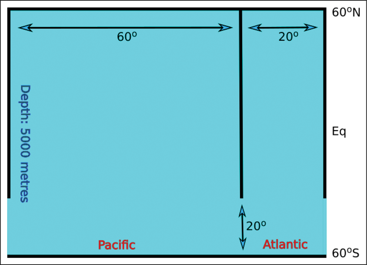
Figure 3
Model domain. Schematic of the two-basin domain with both a large “Pacific” and a small “Atlantic” basin. Single-basin domains are the same as the small basin. Depth is 5000 metres everywhere.
At the ocean surface we restore to an idealised profile of potential temperature (henceforth temperature) and salinity. There is no wind forcing or other mechanical forcing. The restoring profile of temperature has cold water at the northern and southern boundaries, and warm water at the equator. The functional form of this temperature profile is given by
where is the latitude, TS is the temperature at the southern boundary, is the temperature difference between the southern boundary and the equator, and TN is the temperature at the northern boundary. The restoring timescale for temperature is ten days. In all experiments we use , , and .
The restoring profile for salinity has the saltiest water at the equator, and fresher water at the poles. The functional form of this salinity profile is given by
where SS is the salinity at the southern boundary, is the salinity difference between the southern boundary and the equator, and SN is the salinity at the northern boundary. In all two-basin simulations, salinity values in the Pacific basin are set to psu and psu. In all but one single-basin simulation, and in the Atlantic basin in the two-basin simulations, salinity values are set to psu, psu, and psu. The only exception for the single-basin experiments is the one labelled sym in Table 1, which uses a salinity restoring profile symmetric around the equator. In addition, in all model runs labeled ice in Table 1, we use a salinity value of psu at the southernmost grid points, also applied with surface restoring, to simulate brine rejection due to sea ice formation. The restoring timescale for salinity is 30 days. Both temperature and salinity forcing are plotted in Figure 4.
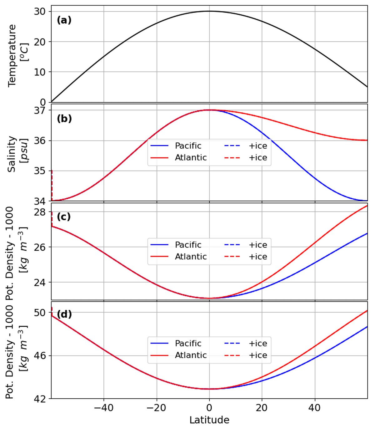
Figure 4
Forcing. (a) Temperature forcing used in all experiments. (b) Salinity forcing for the various experiments and ocean basins. (c) Density calculated from (a) and (b), referenced to the ocean surface. (d) Density calculated from (a) and (b), referenced to the ocean bottom. Differences between (a) and (b) are due to the thermobaric effect. In all single basin experiments, apart from experiment singlebasin_sym, salinity forcing is shown by the red line, and for singlebasin_sym the salinity forcing is shown by the blue line. All two-basin experiments use the salinity forcing shown by the red line for the Atlantic basin and that shown by the blue line for the Pacific basin. If brine rejection by sea ice is simulated in the experiments, salinity at the southern boundary is modified as shown by the red dashed line.
An additional simulation is run with zero planetary rotation, which we label norot in Table 1. Starting with the hydrography from experiment singlebasin, we also run experiments with the same domain and surface forcing, but the depth changed to 1000 m, 2000 m, 3000 m, and 4000 m (experiments singlebasin_1000m - singlebasin_4000m). All simulations are spun-up for the times shown in Table 1, bringing hydrography very close to thermodynamics equilibrium, with mean values shown in this work being calculated over the last 20 years of the experiments. The overturning circulation shown is calculated as a residual overturning on potential density surfaces referenced to 2000 m, and then re-mapped onto depth coordinates.
3 Results
We start with the most “realistic” model configuration to show which features of the global ocean’s overturning circulation can be generated by (rotating) horizontal convection. The flow is generated by just thermohaline surface forcing, in the absence of wind forcing and in the limit of small vertical diffusion. We will then simplify this model configuration step by step to elucidate its dynamics.
The “realistic” thermohaline circulation
The properties of the ocean surface in this “realistic” simulation, experiment twobasin_ice, are shown in Figure 5(a-d), vertical sections of salinity are shown in Figure 6(a,b), and the meridional heat transport is shown in Figure 7(c). The zonal velocities (Figure 5(a)) show a circumpolar current, consisting of multiple zonal jets, in the re-entrant part of the domain. The transport of this circumpolar current is 105 Sv (Sverdrup (Sv) = ), which is slightly below the observed value of the thermal-wind component of the transport of the Antarctic Circumpolar Current of 137 Sv (Meredith et al., 2011). The Atlantic basin shows a northward western boundary current from the northern end of the re-entrant part of the domain to the northern (“Arctic”) limit of the domain. North of about , part of this current heads towards the north-east corner, similar to the North Atlantic Current in the ocean, before heading north as an eastern boundary current in the subpolar gyre.
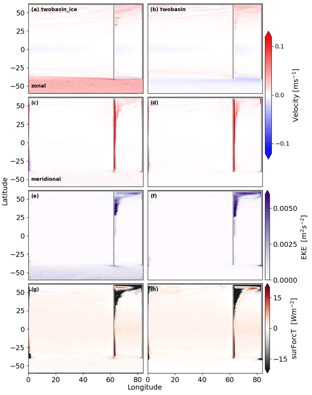
Figure 5
Surface horizontal circulation - two basin. Mean (a,b) zonal velocities , (c,d) meridional velocities , (e,f) eddy kinetic energy , and (g,h) temperature fluxes (positive values show heat uptake into the ocean) at the ocean surface for all two-basin experiments. (a,c,e,g) is for experiment twobasin_ice, and (b,d,f,h) is for experiment twobasin.
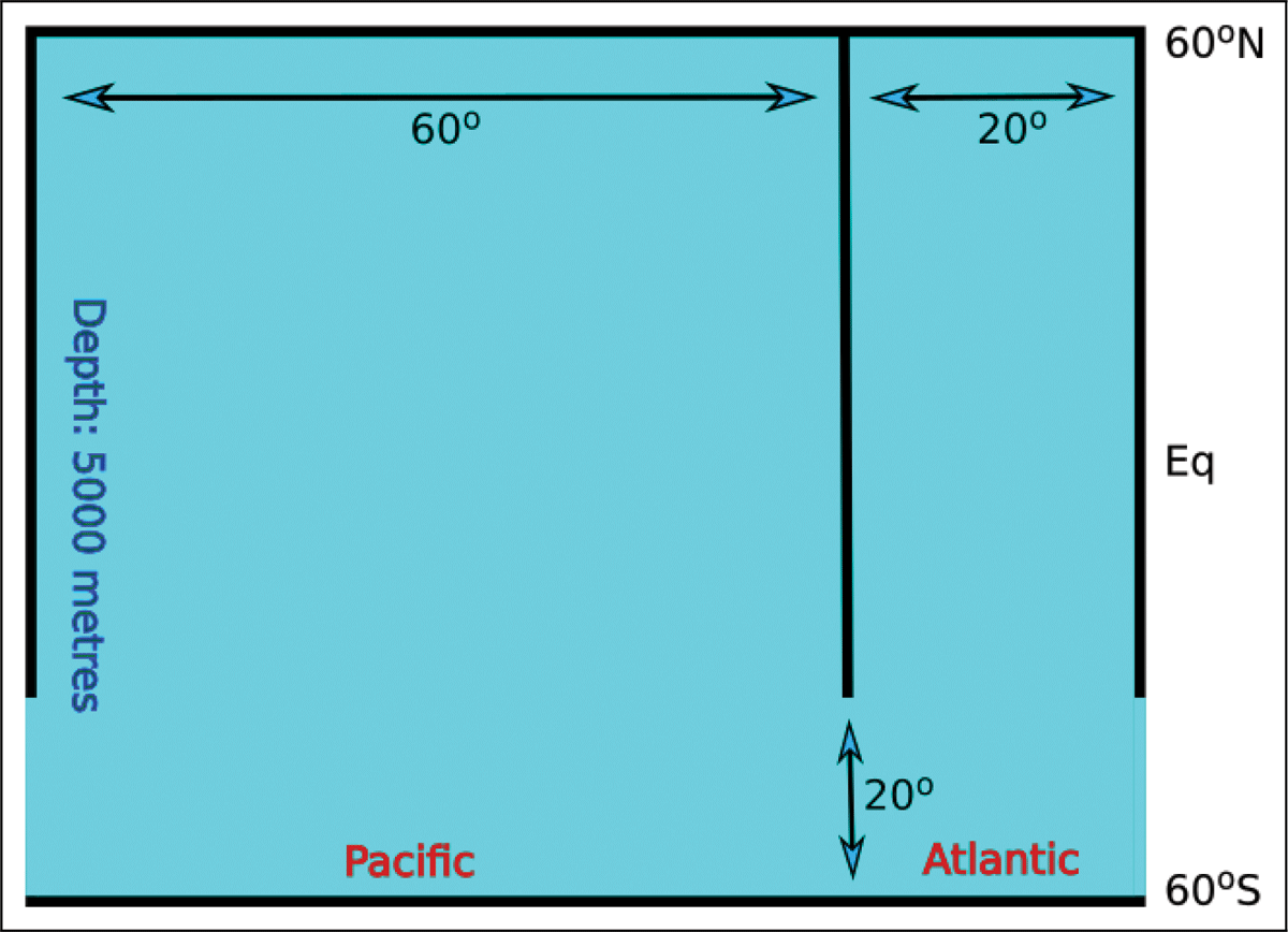
Figure 6
Salinity and overturning circulation in two-basin experiments. Salinity sections and overturning circulation are shown for experiment twobasin_ice in the left row and for experiment twobasin in the right row. Salinity sections are shown along the (a,b) western boundary and (c,d) eastern boundary of the narrow “Atlantic” basin. The overturning circulation is shown integrated across the (e,f) total width of the domain and integrated only across (g,h) the narrow “Atlantic” basin and (i,j) the wide “Pacific” basin, respectively. Green lines show contours of mean potential density referenced to 2000 m, averaged over the respective basins.
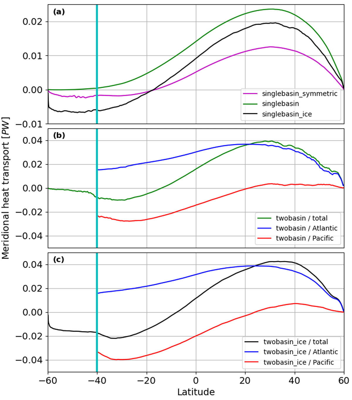
Figure 7
Heat transport. Heat transport for the (a) single basin experiments, (b) experiment twobasin, and (c) experiment twobasin_ice. In (b,c) the two-basin experiments are split into total, Atlantic basin, and Pacific basin. The basin-specific values for the heat transport are masked. The cyan vertical lines show the northern edge of the re-entrant chanel.
Vertical sections of salinity in experiment twobasin_ice, along both the western (Figure 6(a)) and eastern (Figure 6(c)) boundary of the basin, show close similarity to observations (Figure 1). At the surface, we find a warm and salty water mass at low and mid-latitudes. Below this warm and salty surface layer, both the model and observations show cold and fresh AAIW originating in the Southern Ocean. Both the shallow warm and salty water and AAIW move northward as part of the AMOC. Below the AAIW sits the warm and salty NADW generated in the north, providing the southward return flow of the AMOC. This warm and salty water, called Circumpolar Deep Water (CDW) in this region, upwells along the steep isopycnals of the circumpolar current. Adjacent to the bottom we have AABW, which is formed at the southern (“Antarctic”) boundary, feeding the lower overturning cell.
The global MOC in experiment twobasin_ice is shown in Figure 6, both integrated over the entire domain in panel (e), and split into the Atlantic and Pacific basin in panels (g) and (i), respectively. Both upper and lower cells have a maximum overturning circulation of about 4.5 Sv, which, when extrapolated from the narrow basins used in this model configuration to the full width of the global ocean, would be equivalent to a maximum overturning circulation of just over 20 Sv, consistent with observed values (Cessi, 2019). The upper cell, associated with the AMOC, is largely confined to the Atlantic basin, whereas the lower cell is confined to the Pacific basin. The meridional heat transport, shown in Figure 7, is northward in the entire Atlantic basin and largely southward in the Pacific basin. The total heat transport, i.e. integrated over both basins, is northward in the northern hemisphere, and largely southward in the southern hemisphere. These heat transports are consistent in direction, but much weaker in magnitude than observed heat transports (Forget and Ferreira, 2019).
There are two major differences between the idealised model and the observations. The first difference is the thickness of the warm and salty boundary layer at the ocean surface, which is much thinner in the model than in the ocean and can only be seen along the eastern boundary. This is due to the lack of enhanced turbulent vertical diffusivity for the upper oceans in the model, generated by processes such as near-inertial and internal wave activity generated by fluctuating winds; convection due to surface cooling; and brine rejection from evaporation, tides, Langmuir circulation, surface waves, and submesoscale fronts. All of these processes contribute to turbulent mixing in the planetary boundary layer (Moum and Smyth, 2019), enhancing mixing by about two orders of magnitude relative to the vertical diffusivity used here, which would lead to a thickening of the planetary boundary layer (Gayen and Griffiths, 2022). It is this lack of mixing in the thermal boundary layer that is the most likely reason for the heat transport, despite being the right direction relative to observations, being too small compared to the ocean (Klocker et al., 2023a). In addition, large-scale Ekman pumping can thicken the planetary boundary layer, explaining difference between our idealised experiments and the ocean.
The second difference is that in the model the maximum of the overturning streamfunction (Figure 6(e,g)), and the associated upwelling of AAIW and downwelling of warm and salty surface waters (Figure 6(a,c)), occurs against the northern boundary of the domain, while in the realistic ocean this occurs at around N. This difference in location is likely due to the idealised forcing and bathymetry in the model, but given the similarity in the observed water masses, we believe that this should not affect our conclusions.
Sea ice and the Antarctic Circumpolar Current
As a first step towards simplifying this model configuration, in experiment twobasin we show how the modelled overturning circulation changes in the absence of a circumpolar current. To create an ocean circulation without a circumpolar current, we build on results by Klocker et al. (2023a) who show, using purely thermal forcing, how the circumpolar current in the re-entrant part of the domain is intimately linked to convection at the southern (“Antarctic”) boundary. In particular, the circumpolar current is similar to a rim current that develops around a site of deep convection, which for convection in a re-entrant domain such as the Southern Ocean takes the form of a circumpolar current. Convection against the southern boundary, and hence the circumpolar current, can therefore only exist in an equilibrated ocean if the densest water in the domain is produced south of the circumpolar current (Klocker et al., 2023a).
In the experiments shown here, if the salinity at the northern boundary is sufficiently salty to generate an AMOC with properties similar to those observed in the ocean, the density at the northern boundary will exceed that at the southern boundary. This is shown in Figure 4c, which translates the surface restoring conditions for temperature and salinity to density. We achieve the necessary condition of a denser southern boundary in experiment twobasin_ice by simulating brine rejection due to sea-ice formation at the south with an elevated SS (Figure 4(b); blue dashed line). While the resulting potential density, when referenced to the ocean surface (Figure 4(c)), is still denser at the northern boundary, the potential density referenced to the ocean bottom (Figure 4(d)) is now densest at the southern boundary. This difference in potential densities between ocean surface and ocean bottom is due to the thermobaric effect, a result of the nonlinear equation of state of seawater, and is large enough to ensure that the densest water mass is formed at the southern boundary. Once we take away this brine rejection, as done in experiment twobasin, we lose both southern convection and the circumpolar current as the southern boundary now forms water with a reduced salinity. In this case, the water formed at the northern boundary is denser than that formed at the southern boundary. This prevents the northern source water from upwelling at the southern boundary and it must turn northwards at intermediate depths to return northwards and obduct into the surface layers north of the channel. This contrasts with experiment twobasin_ice in which the northern source water is of density intermediate between the southern boundary and the northern edge of the channel.
In the case of experiment twobasin the isopycnals below ~500 m slope upwards to the north (Figure 6(f,h,j); green lines), which produces a westward thermal wind shear. This contrasts with the typical Southern Ocean configuration of isopycnals sloping steeply downwards to the north, achieved by experiment twobasin_ice (Figure 6(e,g,i); green lines), which produces an eastwards thermal wind shear. As a result of the change in sign of the across-channel density gradient in twobasin westwards flow persists over most of the north-south extent of the channel at most depths. As shown in Figure 5 there is some intense eastwards flow at the northern edge of the channel near the tip of the land barrier between the Pacific and Atlantic basins. This is due to routing of the flow on the northern edge through the constrictions. Above ~500 m, the water on the northern side of the channel begins to warm because of the surface restoring condition, and this offsets the continued northwards salinity gradient. As a result, the density difference across the channel changes sign and so does the thermal wind shear, which results in the westward thermal wind shear in the bottom deep ocean being closely offset by the eastwards thermal wind shear in the near surface. The result is a near zero circumpolar transport. In experiment twobasin, the dense water formation in the north of the Atlantic basin is therefore enough to stop any southern convection, whether in the Atlantic or Pacific basin, and hence the formation of a circumpolar current.
The properties of the ocean surface in experiment twobasin are shown in Figure 5(b,d,f,h), vertical sections of salinity are shown in Figure 6(b,d), and the meridional heat transport is shown in Figure 7. In agreement with the thermally-driven simulations by Klocker et al. (2023a), the zonal velocities (Figure 5(b)) show that there is no circumpolar current. Despite the absence of the circumpolar current, zonal velocities (Figure 5(b)), meridional velocities (Figure 5(d)), eddy kinetic energy (Figure 5(f)), and surface temperature fluxes (Figure 5(h); positive values show heat uptake into the ocean) are very similar everywhere north of the re-entrant channel between experiments twobasin_ice and twobasin. The only minor difference is that in experiment twobasin, the circulation in the closed part of the domain is slightly stronger, possibly due to the circulation adjusting to a near-zero southward heat transport across the circumpolar current (Figure 7). In the vertical, as seen by the vertical salinity sections, the only major difference between experiment twobasin_ice (Figure 6(a,c)) and twobasin (Figure 6(b,d)) is the presence of AABW below about 4000 m, as expected from the link between convection, AABW formation, and the circumpolar current.
The MOC integrated over the entire domain for this experiment is shown in Figure 6(f), and split into the Atlantic and Pacific basin in Figure 6(h) and 6(j), respectively. The upper overturning cell, associated with the AMOC, can therefore exist without a circumpolar current, and becomes about twice as strong for that case. This shows that upwelling along steep isopycnals across the circumpolar current is not necessary to close the upper overturning cell. Instead, looking at the overturning streamfunction in Figure 6, this overturning circulation seems to be closed by upwelling in the convection region against the northern boundary. This strengthening of the overturning will be discussed more below.
Overturning in a single vs. two-basin ocean
Next, we focus on the role of the second, or Pacific, basin on the global ocean’s overturning circulation. To this end, we run two additional simulations with a single Atlantic basin. These experiments have the same forcing as the Atlantic basins in experiments twobasin_ice and twobasin, but without the larger Pacific basin, and are called singlebasin_ice and singlebasin, respectively.
Similar to its two-basin equivalents, the simulation of brine rejection due to sea ice production at the southern boundary in experiment singlebasin_ice leads to convection at the southern boundary with an associated circumpolar current (Figure 9(a)), the formation of AABW (Figure 8(a,c)), a lower overturning cell (Figure 8(e)), and a southward heat transport across the re-entrant channel (Figure 7(a); black line). In experiment singlebasin, on the other hand, neither convection, a circumpolar current (Figure 9(a)), the formation of AABW (Figure 8(b,d)), a lower overturning cell (Figure 8(f)), nor a southward heat transport across the re-entrant channel (Figure 7(a); green line) exist. As in the two-basin equivalent, the dynamics north of the re-entrant channel change very little between experiments singlebasin and singlebasin_ice (Figure 9(a–d) vs. Figure 9(e-h)), and the upper overturning cell associated with the AMOC becomes about twice the strength (Figure 8(e) vs. (f)) and the northward heat transport increases (Figure 7; black line vs. green line).
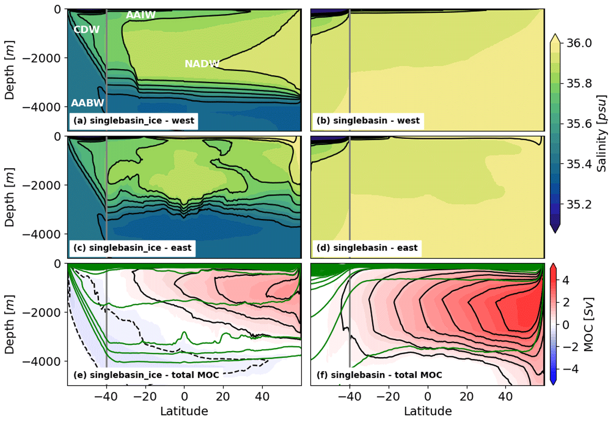
Figure 8
Salinity and overturning circulation in single-basin experiments. Salinity sections and overturning circulation are shown for experiment singlebasin_ice in the left row and for experiment singlebasin in the right row. Salinity sections are shown along the (a,b) western boundary and (c,d) eastern boundary of the domain. (e,f) The overturning circulation is shown integrated across the total width of the domain. Green lines show contours of mean potential density referenced to 2000 m, averaged over the respective basins.
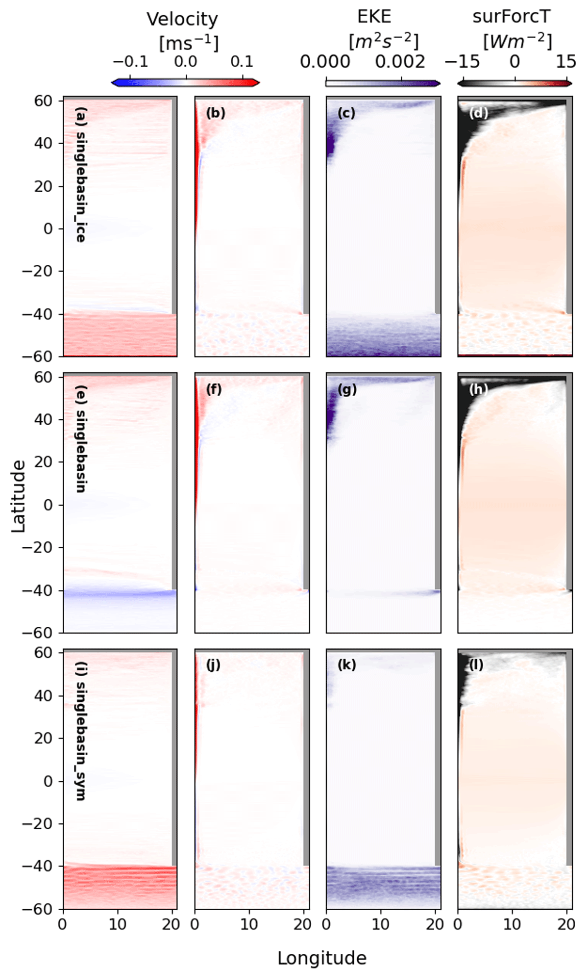
Figure 9
Surface horizontal circulation - single basin. Mean (a,e,i) zonal velocities , (b,f,j) meridional velocities , (c,g,k) eddy kinetic energy , and (d,h,l) temperature fluxes at the ocean surface (positive values show heat uptake into the ocean) for all single basin experiments. (a-d) is for experiment singlebasin_ice, (e-h) is for experiment singlebasin, and (i-l) is for experiment singlebasin_sym.
The main change between the single- and two-basin experiments is seen in the western boundary current in the Atlantic basin. In the two-basin experiments, the western boundary current in the Atlantic basin is northward everywhere in the blocked part of the domain, that is, everywhere north of the re-entrant channel. In the single-basin experiments, on the other hand, the western boundary current is northward north of S, and southward south of S. This direction of the western boundary current, from low to high latitudes, is very similar to that simulated for purely thermally-generated flows in the same domain (Klocker et al., 2023a; Xing et al., 2023), and can be explained by horizontal convection where the surface flow is from heated to cooled regions (Gayen and Griffiths, 2022; Hughes and Griffiths, 2008). The combination of a second basin, or “Pacific” basin, together with the saltier “Atlantic” basin therefore allows for a tipping of the circulation from being symmetric around the equator, with flow from low to high latitudes, to a circulation where the heat transport is northward in the entire Atlantic basin.
The change in water mass structure resulting from the existence of a second basin can be seen from vertical salinity sections along the western and eastern boundaries in the Atlantic basin (Figure 6(a-d) vs. Figure 8(a-d)). Independent of convection in the south, the western boundary current in the two-basin experiments advects cold and fresh water from the surface Southern Ocean towards the north, leading to a cold and fresh AAIW layer between the warm and salty surface layer and the warm and salty NADW. In the single-basin experiments, on the other hand, the western boundary current is southward in the southern hemisphere, and hence not transporting cold and fresh water from the surface Southern Ocean towards the north. The cold and fresh AAIW in the two-basin experiments therefore leads to a much stronger salinity contrast between the warm and salty surface waters and NADW on one hand, and the cold and fresh AAIW on the other. The AAIW upwells just south of the northern boundary where it is visible as a positive temperature flux (Figure 5(d,h); positive values show heat uptake into the ocean).
Asymmetrical salinity forcing
One key ingredient required to simulate a realistic-looking AMOC in our simulations is to use salinity restoring, in which the salinity values adjacent to the northern boundary are higher than over the re-entrant channel. To understand the role of this asymmetric salinity forcing, and to compare to the pure thermally-forced experiments by Klocker et al. (2023a), we now look at a single-basin experiment in which salinities are symmetric around the equator - experiment singlebasin_sym. Note that due to the form of the surface salinity restoring condition, which places the peak salinity at the Equator, none of the models produce low Tropical salinities. Our focus here is upon the subsurface hydrography and stratification, rather than the surface values, which are well simulated in our more realistically-forced models.
As the southern-most latitude is now the densest part of the ocean, even without the simulation of brine rejection due to the southern boundary being colder, there is convection at the southern boundary. The horizontal flow (Figure 9(i)) shows a circumpolar current, with a transport of 73 Sv, and the overturning has an upper and lower cell structure with AABW formation near the southern boundary (Figure 10(c)). The vertical salinity sections (Figure 10(a,b)) agree with the thermally-forced results of Klocker et al. (2023a) who show that the stratification to the north of the re-entrant channel is set through a projection of the surface gradient across the circumpolar current along sloping isopycnals towards the north; this is exactly what is seen by the northward projection of the cross-channel salinity gradient.
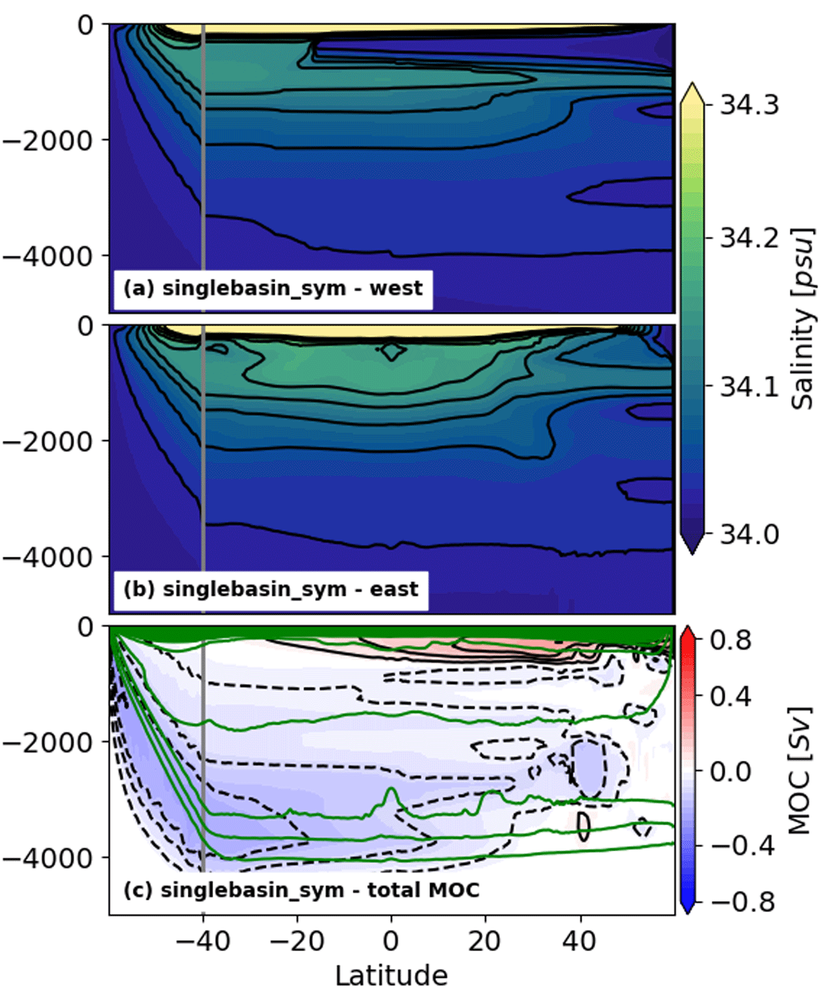
Figure 10
Salinity and overturning circulation for symmetrical salinity forcing. Salinity sections and overturning circulation are shown for experiment singlebasin_sym. Salinity sections are shown along the (a) western boundary and (b) eastern boundary of the basin. (c) The overturning circulation is shown integrated across the total width of the domain. Green lines show contours of potential density referenced to 2000 m.
The overturning circulation in experiment singlebasin_sym (Figure 10(c)) is much weaker than in the asymmetric experiments, consistent with a much weaker heat transport (Figure 7; magenta line), and is almost exactly the same as in the thermally-forced experiments of Klocker et al. (2023a). The shallow upper cell now advects relatively fresh water southwards, as seen in Figure 10(a,b), as opposed to the saline NADW in all experiments with asymmetric salinity forcing. This water mass remains too light/fresh to deepen the northern boundary convection, and the overturning cell is therefore much weaker than in the experiments with asymmetric salinity forcing. Consistent with this weaker upper overturning cell is the weaker horizontal circulation north of the re-entrant channel (Figure 9(i-l)). These results show that both AAIW and NADW are therefore a consequence of asymmetric thermal and haline forcing, with cold and fresh AAIW formed in the south, and warm and salty NADW formed in the north. Neither AAIW nor NADW can exist without its counterpart.
Linking convection depth and overturning strength
One point that becomes evident in all the model experiments explained above is that if a lower overturning cell exists, constraining the upper cell to a shallower depth—the upper cell becomes substantially weaker. In singlebasin_sym, where northern convection is the shallowest, the upper cell is also the weakest. To further test the relationship between convection depth and overturning strength we now look at additional experiments, starting with experiment singlebasin, which only produces an upper overturning cell due to a lack of convection at the southern boundary, and reduce the depth of the model domain to 4000 m, 3000 m, 2000 m, and 1000 m (experiments singlebasin_4000m to singlebasin_1000m).
As shown in Figure 11, in these experiments, which all convect full depth, the maximum overturning is linearly dependent on convection depth. Deeper convection therefore leads to a stronger overturning circulation, despite the same surface forcing, at least for the upper overturning cell in the closed basin, i.e. the AMOC. We also add the other singlebasin experiments that generate a lower overturning cell to this figure. These results (orange dots in Figure 11) show that the maximum in the overturning streamfunction is slightly lower than expected from the scaling generated by the experiments with just an upper overturning cell. This is likely due to the fact that if a lower overturning cell exists, heat transport to the southern boundary increases, reducing the northward heat transport and hence the overturning strength of the upper cell. Nevertheless, these experiments suggest a strong dependency of overturning strength on convection depth.
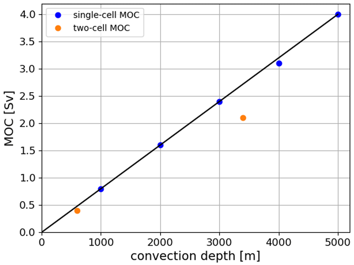
Figure 11
Convection depth vs. overturning strength. Strength of the overturning relative to convection depth is shown for all single-basin experiments. Blue dots show experiments that produce a single overturning cell, and orange dots show experiments that produce two overturning cells.
Planetary rotation, boundary currents and eddies
We now take one final step to further simplify the circulation dynamics in the narrow “Atlantic” basin by running experiment singlebasin_ice_norot, which is equivalent to experiment singlebasin_ice in the absence of planetary rotation. That is, we simulate horizontal convection generated by thermal and haline forcing, rather than rotating horizontal convection. We therefore eliminate the geostrophic constraints on the planetary boundary layer and the interior flows, such as the boundary currents that are important for meridional heat transport, and the baroclinic eddies, which add to the release of available potential energy and the heat transport across the re-entrant channel.
The resulting horizontal circulation of experiment singlebasin_ice_norot is shown in Figure 12, and the vertical circulation in Figure 13. Due to the lack of rotation, the re-entrant channel loses its dynamic significance; there is no longer a geostrophic constraint requiring a zonal pressure gradient to allow meridional flow. The meridional flow is in the same direction as in the rotating case, but its velocity is about two orders of magnitude larger. This is consistent with the stronger surface fluxes and the theoretical understanding that geostrophy constrains the flow (Park and Whitehead, 1999; Vreugdenhil et al., 2017) with the larger surface fluxes. The planetary boundary layer at the surface becomes thinner in the non-rotating experiment (Gayen et al., 2014), and both “endwall” convection and downwelling occur homogeneously distributed along the northern and southern boundaries. Despite these differences, which are all consistent with theory and experimental evidence (Gayen and Griffiths, 2022), the layering of water mass structure is still similar to the rotating case, (Figure 13(c) vs. (d)), in that the circulation leads to a thin warm and salty surface layer, cold and fresh AAIW below, followed by NADW even deeper, and an AABW layer adjacent to the bottom. Nevertheless, the differences in temperature and salinity between the different layers are much smaller, likely due to the surface restoring acting on a much stronger flow. These results show that while geostrophic dynamics make the flow more complicated through the presence of boundary currents, eddies, and the dynamics of a re-entrant channel, the water mass structure we observe in the Atlantic basin can be explained by simple horizontal convection generated by asymmetric thermal and haline forcing.
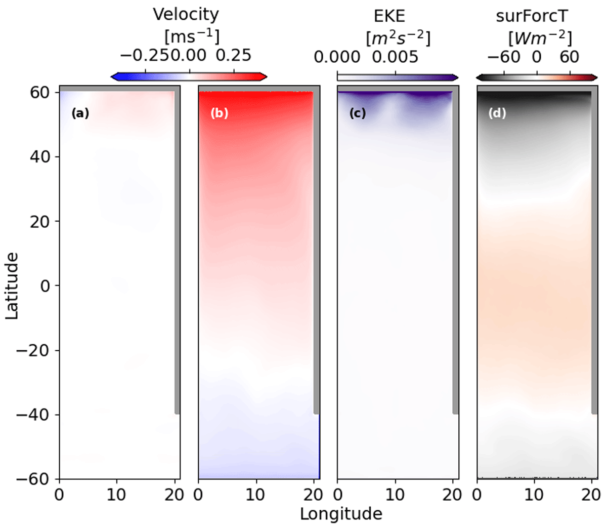
Figure 12
Surface horizontal circulation - singlebasin norot. Mean (a) zonal velocities , (b) meridional velocities , (c) eddy kinetic energy , and (d) temperature fluxes at the ocean surface (positive values show heat uptake into the ocean) for experiment singlebasin_sym.
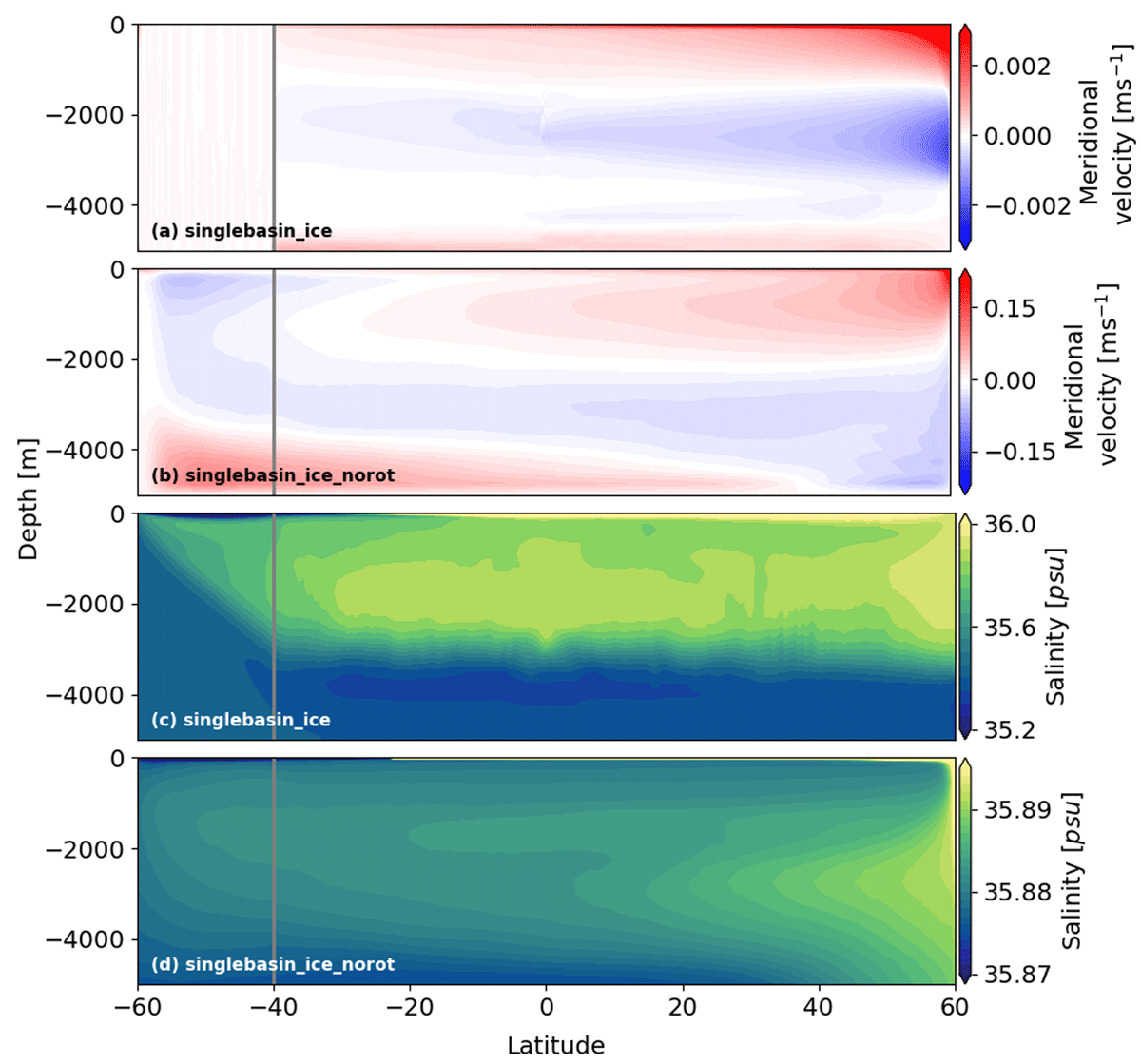
Figure 13
Vertical circulation - effect of planetary rotation. (a,b) Zonal mean meridional velocities, and (c,d) zonal mean salinities for (a,c) experiment singlebasin_ice and (b,d) experiment singlebasin_norot.
4 Discussion
Using an idealised eddying ocean model, we have shown that thermal and haline forcing alone, without winds and in the limit of small vertical diffusion, can generate an overturning circulation and a water mass structure that closely resembles that of the global ocean. Due to only being generated by thermal and haline forcing, this could be identified as what is often called the “thermohaline circulation”. This is consistent with arguments by Wyrtki (1961) that only thermohaline processes can explain the formation of different water masses and the distribution of density in the ocean. It opposes the view that tidal stirring and a wind-driven upwelling are required to generate such a strong overturning circulation with the structure observed in the global ocean (Wunsch, 2002).
Our results build on the work by Klocker et al. (2023a) who used a similar model configuration, but forced solely by thermal forcing, to show that buoyancy forcing alone can lead to a full-depth two-cell overturning circulation. Adding haline forcing, and a second larger ocean basin representative of the Pacific, we are now able to simulate the main features of the global ocean’s overturning circulation, which could not be reproduced with just thermal forcing. In the Atlantic basin, these features include the northward moving warm and salty layer at the ocean surface and the cold and fresh AAIW below, balanced by the southward moving warm and salty NADW layer below. These layers are all part of the upper overturning cell, or AMOC. In the thermally-forced experiments of Klocker et al. (2023a), this upper cell was much shallower and weaker than in the results shown here. These changes could be either due to the combination of thermal and haline forcing, the nonlinear equation of state, or likely a combination of both these changes. Below the upper cell we find the lower cell associated with cold and fresh AABW, confined largely to the Pacific basin. That is, at least within the limitations of a primitive equation ocean model with parameterised convection and some numerical diffusion, rotating horizontal convection can generate a full-depth thermohaline circulation with the water mass structure very similar to that observed in the real ocean.
While both upper and lower overturning cells can exist independently of each other, as shown by Klocker et al. (2023a) for the lower cell and the experiments presented here for the upper cell, one feature that only exists in the presence of both overturning cells is the warm and salty tongue across the re-entrant channel, the model equivalent of CDW upwelling. This upwelling of CDW is generally associated with wind-driven upwelling in the Southern Ocean (Marshall and Speer, 2012). As shown here though, the upwelling of CDW can be generated by horizontal convection alone, and can be explained as follows. In the model, we force the initiation of southern boundary convection by increasing the salinity at the boundary in a gross simplification of brine rejection by sea-ice freezing. The region to the north of the boundary remains fresh in a gross simplification of sea-ice melting. This is a very simple way of simulating sea-ice processes in the real ocean where the formation, export and melting of sea-ice increases salinity at the coast, reduces the salinity further north, and hence widens the salinity contrast between AABW and AAIW. This enhanced salinity contrast creates a “shared buoyancy window” (Wolfe and Cessi, 2011, 2014) between dense water masses formed in the north, the NADW, and the density gap between AAIW and AABW in the south. This shared buoyancy window allows for NADW to upwell adiabatically in the Southern Ocean, instead of returning to the northern boundary as in our experiments without “sea-ice”. This link between sea-ice and the global overturning circulation is consistent with estimates of water mass transformation using the Southern Ocean state estimate (Abernathey et al., 2016) and observations (Pellichero et al., 2018), and the quantitative link between the melting and freezing of sea ice, and mid-depth stratification, shown in a realistic ice-ocean model by Klocker et al. (2023b). Southern Ocean upwelling of CDW therefore likely provides a link between the upper and lower overturning cells, and its exact role in this two-cell overturning system will have to be tested in future work using eddying model simulations. One possible outcome of such work could be that winds in the Southern Ocean set the relative balance between these two routes.
The results summarised above show that in addition to the need for an asymmetric thermal forcing at the ocean surface, as discussed by Klocker et al. (2023a), the generation of an overturning circulation and water mass structure similar to observations also requires asymmetric surface salinity between the (sub)polar regions. In our experiments, this is forced directly by asymmetric surface salinity restoring conditions. However, in models with surface freshwater or salt fluxes, this asymmetry can arise via salt advection feedbacks, which are one source of multiple equilibria of the ocean circulation (Huisman et al., 2009; Stommel, 1961; Wolfe and Cessi, 2014). Such asymmetry allows the formation of a salty North Atlantic and a fresh Southern Ocean, and the formation of salty AABW by brine rejection at the southern (“Antarctic”) convective regions, that nevertheless have overlapping density ranges that allow for flow between them at steady state/equilibrium. Without such an asymmetry, neither warm and salty NADW nor cold and fresh AAIW are formed, as confirmed by the model results using symmetric salinity forcing. Our results therefore show a tight coupling between NADW and AAIW, such as suggested from ocean circulation changes in Earth’s past as reconstructed by proxies (Pahnke, 2005; Pahnke et al., 2008), and with model experiments showing hysteresis of the Atlantic’s overturning circulation as a consequence of having either NADW or AAIW denser than one another (Saenko et al., 2003; Stouffer et al., 2007). These results are also consistent with several model studies that show the importance of pole-to-pole density differences in setting up an asymmetric overturning circulation, and as the cause for multiple equilibria (Hughes and Weaver, 1994; Klinger and Marotzke, 1999; Marotzke and Willebrand, 1991; Rahmstorf, 1996), even with symmetrised surface fluxes forcing the salinity.
One of the unique features of the Atlantic basin in the real ocean is that heat transport is northward along all latitudes. This northward heat transport means that in the South Atlantic heat transport is up-gradient, from high latitudes towards the equator. This is opposite to all examples of horizontal convection where the flow is from the heated regions around equatorial latitudes to the cooling regions in high latitudes. This northward flow in the Atlantic basin can only be reproduced in the presence of two basins, with the north of the Atlantic basin being saltier than the north of the Pacific basin. The result of this northward flow is that AAIW advects cold and fresh water mass properties from the Southern Ocean towards the north, leading to a much more prominent water mass contrast between warm and salty surface waters, cold and fresh AAIW, and warm and salty NADW.
From an overturning point of view, the MOC integrated over the entire model show s a two-cell overturning circulation, with a clockwise overturning cell sitting above an anti-clockwise overturning cell, for both the single-basin or two-basin experiments. Nevertheless, in the two-basin experiments, integrating the MOC over both basins separately shows that these two overturning cells are now separated into their respective basins; the Atlantic basin shows a clockwise overturning circulation consistent with the northward flow and heat transport, whereas the Pacific basin shows a counter-clockwise overturning circulation. Interestingly, this split into clockwise and counter-clockwise cells with two basins is also the case for the experiments without convection at the southern boundary, i.e. experiments that only show a single clockwise overturning cell in the global integral.
We have shown that most of the observed water mass structure in the ocean can be generated by horizontal convection. Part of this global circulation due to horizontal convection is the vertical, or upright, convection against the endwall, the idealised equivalent of deep convection observed in the Irminger and Labrador basins. To understand the role of this endwall convection in setting the strength of the overturning circulation, we conducted additional experiments in which we changed the maximum convection depth by (a) changing the depth of the model domain, and (b) comparing experiments in which the convection depth was modified by the presence of a lower overturning cell. These results show that, at least for changes in domain depth, there is a clear linear relationship between convection depth and overturning strength, highlighting the role of deep convection in setting the strength of the ocean’s overturning circulation. In the presence of a lower cell the behaviour is very similar, but with an overturning strength slightly reduced compared to the same convection depth achieved by changing the domain depth, which is likely due to interaction between the two cells through a shared buoyancy window. These results might at first sight seem strange when considering the scaling arguments of Klocker et al. (2023b), which do not show a dependency of overturning strength on ocean depth. This can be explained by the assumptions that went into these scaling arguments in which the overturning strength depends only on properties of the thermal boundary layer and surface forcing. Nevertheless, overturning strength also depends on the potential energy released through convection, which itself is proportional to convection depth (Gayen et al., 2014). The effect of convection depth on overturning strength has seen very little attention in the literature on horizontal convection, pointing towards the need for future work in that direction.
Last but not least, we tested how the overturning circulation changes in the absence of planetary rotation, that is, how much of the overturning circulation can be explained using the framework of horizontal convection rather than rotating horizontal convection. Without planetary rotation, the circumpolar current, the meridional boundary currents and mesoscale eddies disappear, and the meridional flow now occurs homogeneously across the domain. In these experiments the meridional flow and the overturning circulation become much stronger, as expected from theory and from turbulence-resolving direct numerical simulations that show how planetary rotation constrains the flow (Gayen and Griffiths, 2022). Despite being forced in the same way as its rotating counterparts, the non-rotating experiments produce a much weaker temperature and salinity contrast between water masses, but a similar layering of warm/salty and cold/fresh water masses.
The crucial role of (rotating) horizontal convection in the overturning circulation has important consequences for the development of parameterisations of small-scale processes not resolved by ocean models. While in the past much effort has been devoted to developing parameterisations of vertical mixing by winds and tides, the dominant role of horizontal convection in the ocean’s global overturning circulation points towards the need to focus on the parameterisation of the planetary boundary layer and deep convection. Given that in horizontal convection the strength of the flow is controlled by processes in this planetary boundary layer, all of which cannot be resolved in global ocean models, an accurate representation of these small-scale processes is extremely important, especially when the goal of these ocean models is to accurately predict future changes in the overturning circulation. Currently, convection in ocean models is parameterised such that it vertically mixes the water column in the presence of static instability. This is a huge oversimplification of the processes setting the strength of the global ocean’s overturning circulation and may have implications for the sensitivity of the circulation as whole to changes in surface forcing, such as we might expect under anthropogenic climate change.
Data Accessibility Statement
The model output can be provided by AK, and requests for the model output should be submitted to ankl@norceresearch.no.
Acknowledgements
AK appreciates the support of the Bjerknes Centre for Climate Research through its backing from the Norwegian Ministry of Education and Research, and he thanks his colleagues at the Bjerknes Centre’s DYNASOR (DYnamics of the North Atlantic Surface and Overturning ciRculation) project for useful discussions.
Competing Interests
The authors have no competing interests to declare.