
Figure 1
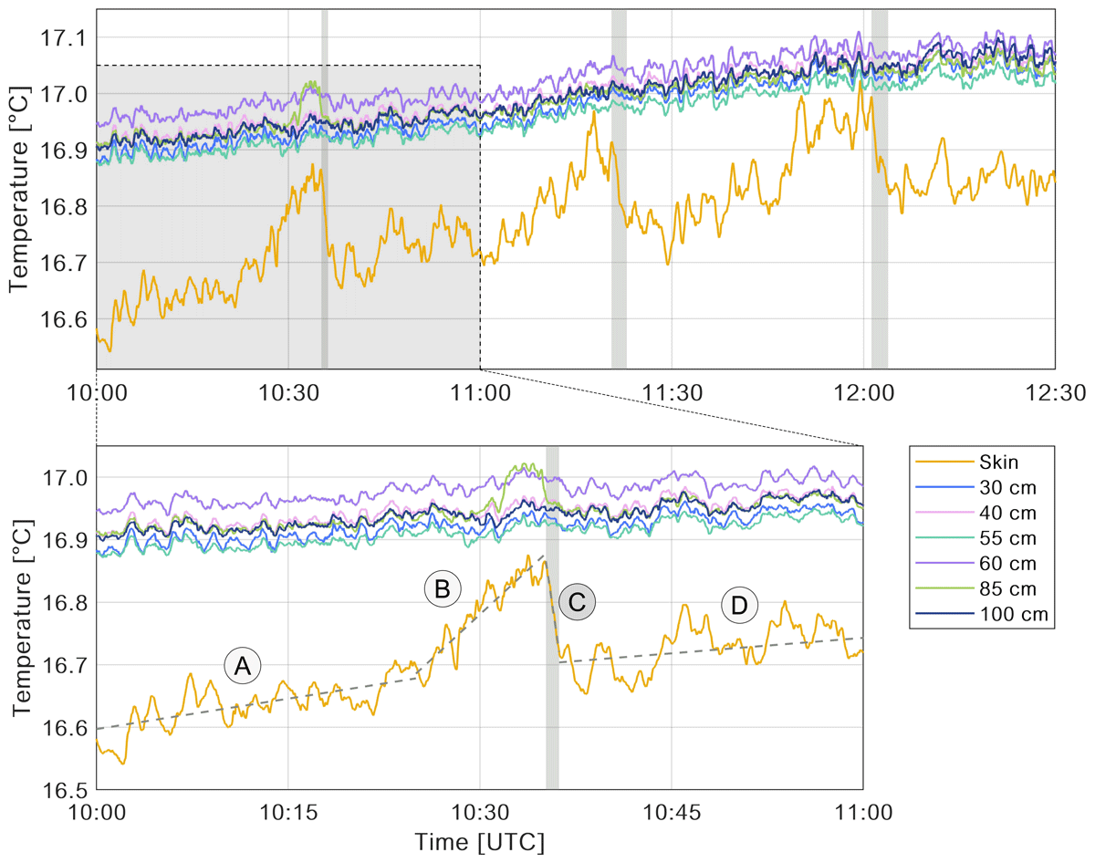
Time series of temperature in the skin and near-surface layer at various depths during three artificial disturbances of the ocean’s surface (top) and zoomed time series of the first disturbance (bottom). Dashed lines are temperature regression lines of the skin layer for phases: (A) before disturbance, (B) during disturbance, (C) recovery of the thermal skin layer, and (D) after recovery. Gray bars represent the duration of thermal skin recovery. (Zoomed time series for disturbances two and three see Figure S3.)
Table 1
Time of the onset of the recovery phase, skin layer recovery times (t*), skin temperatures before (Tskin start) and after recovery (Tskin end), skin temperature difference (Tskin diff), and temperature anomalies before and after recovery (ΔT = Tskin – T100 cm) for each of the three disturbances.
| TIME UTC [hh:mm:ss] | t* [s] | Tskin START [°C] | Tskin END [°C] | Tskin DIFF [°C] | ΔT START [°C] | ΔT END [°C] | |
|---|---|---|---|---|---|---|---|
| 1st Disturbance | 10:35:10 | 62 | 16.861 | 16.721 | 0.140 | –0.086 | –0.229 |
| 2nd Disturbance | 11:20:32 | 144 | 16.914 | 16.764 | 0.150 | –0.103 | –0.248 |
| 3rd Disturbance | 12:01:12 | 157 | 16.995 | 16.833 | 0.162 | –0.060 | –0.217 |
Table 2
Temperature rates in °C min–1 for phase A-D which are shown as regression lines in Figure 1 and Figure S3. The recovery rates (Rt) of the cool-skin layer are highlighted in bold.
| BEFORE (A) | DISTURBANCE (B) | RECOVERY (C) | AFTER (D) | |
|---|---|---|---|---|
| 1st Disturbance | 0.003 | 0.019 | –0.140 | 0.002 |
| 2nd Disturbance | 0.002 | 0.013 | –0.070 | 0.003 |
| 3rd Disturbance | 0.003 | 0.052 | –0.047 | 0.000 |
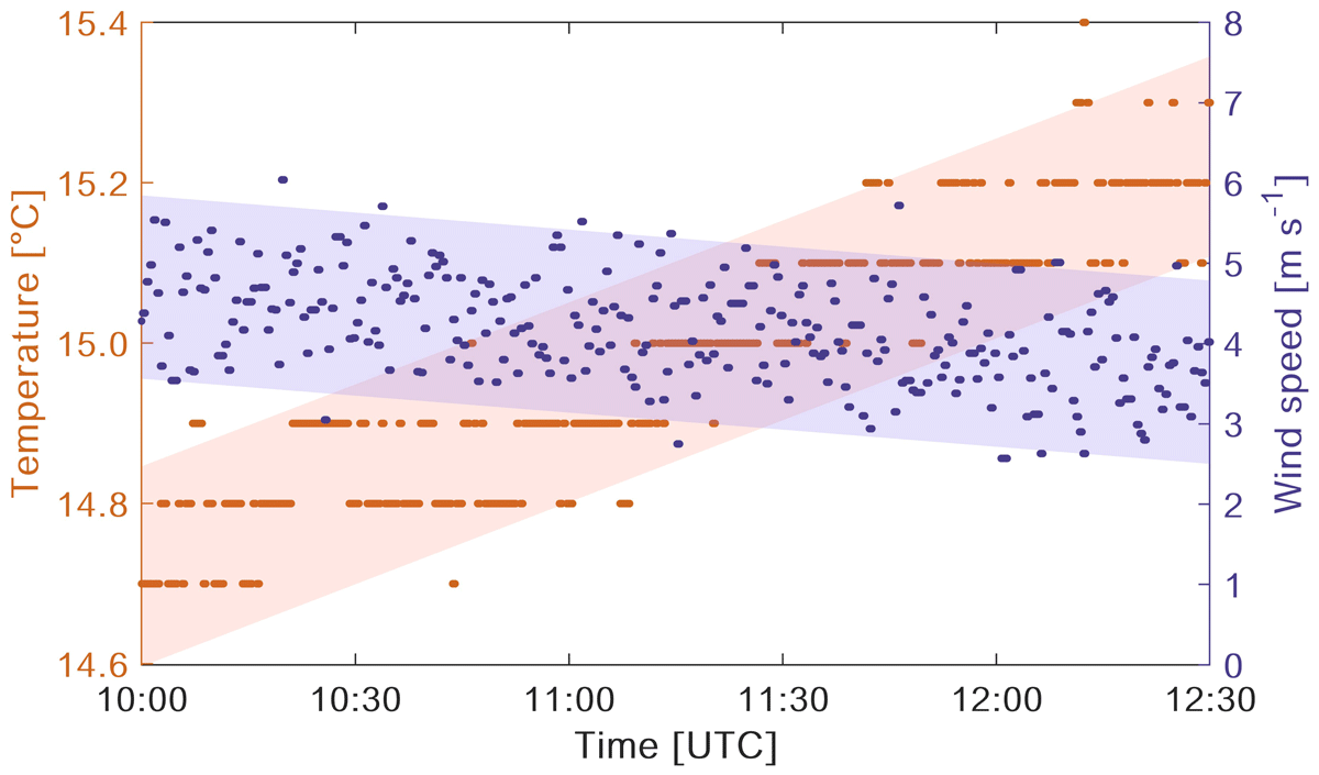
Figure 2
Air temperature (red) and wind speed (blue) recorded during the experiment by the autonomous surface vehicle Halobates. The shaded area represents a 95% prediction interval for the estimated regression lines.
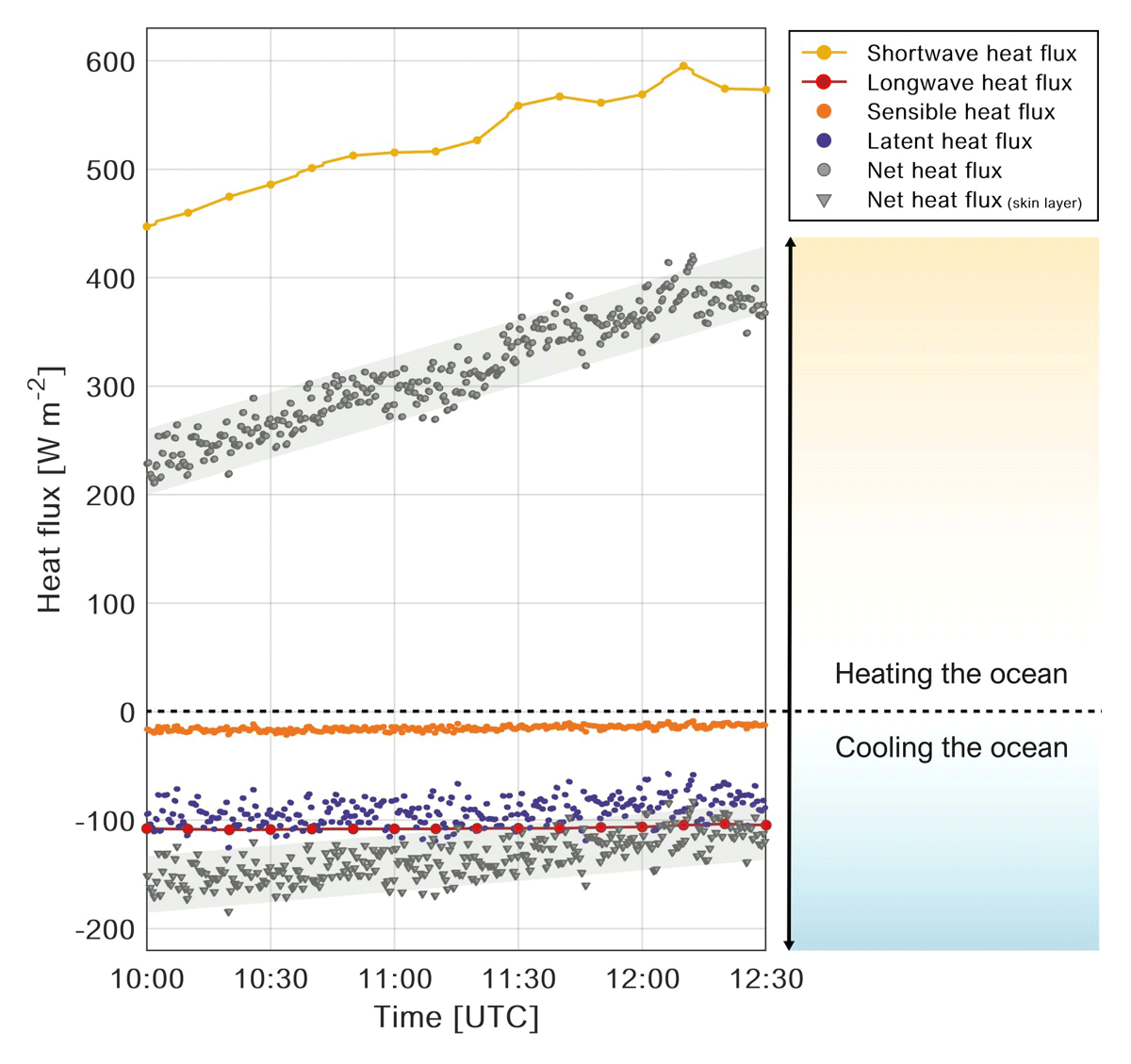
Figure 3
Components of the air-sea heat flux: Shortwave heat flux (yellow line) calculated based on measurements of incoming shortwave radiation (yellow dots). Longwave heat flux (red line) calculated based on measurements of downwelling and upwelling longwave radiation (red dots). Sensible (orange) and latent heat flux (blue) calculated using the COARE 3.6 algorithm (Fairall et al. 2003). Gray dots represent net air-sea heat flux, while gray triangles represent the net heat flux of the skin layer (approx. 1 mm). The shaded area represents a 95% prediction interval for the estimated regression lines.
Table 3
Net heat flux in the skin layer QN skin, recovery temperature change ΔTτ for recovery times t*, and the restoring internal energy flux Jr for each of the three disturbances.
| QN skin [W m–2] | ΔTτ(t*) [°C] | Jr [W m–2] | |
|---|---|---|---|
| 1st Disturbance | –147.61 | 0.846 | 10.15 |
| 2nd Disturbance | –132.58 | 1.158 | 5.07 |
| 3rd Disturbance | –119.19 | 1.087 | 3.41 |
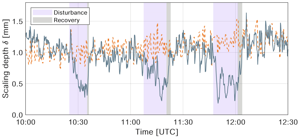
Figure 4
Comparison between the calculated scaling depths of the thermal skin layer from a bulk formula by Katsaros (1980) (blue line) and the thickness of the skin layer calculated with the COARE 3.6 algorithm (dashed orange line). Shaded areas indicate periods of artificial disturbance and the subsequent recovery.