
1. Introduction
The skin layer is the uppermost layer of the ocean, typically less than 1 mm thick, and is characterized by temperature (ΔT = Tskin – Tbulk) and salinity anomalies (ΔS = Sskin – Sbulk) compared with the bulk phase (Donlon et al. 2002; Gassen et al. 2024; Jessup and Branch 2008). These anomalies are driven primarily by net heat flux and wind-induced mixing, which often result in a cooler skin layer with temperature differences of several tenths of degree Celsius (Murray et al. 2000; Wurl et al. 2019; Yan et al. 2024). This cooling effect significantly influences gas solubilities (Watson et al. 2020). As a significant sink for anthropogenic carbon dioxide, the ocean’s carbon uptake is notably influenced by the cool-skin layer. When accounting for its effect, the oceanic carbon uptake increases substantially, with the global annual uptake rising from 2.0 petagrams of carbon per year to a minimum of 2.8 petagrams (Watson et al. 2020). Donlon et al. (1999) found that the variability of temperature anomalies (ΔT) decreases with increasing wind speed, as the skin temperature becomes more closely coupled to the temperature of the underlying water. The authors found a typical temperature anomaly of –0.14 ± 0.10°C when wind speeds exceeded 6 m s–1. With an average wind speed of 6.6 m s–1 over the ocean (Archer and Jacobson 2005), it can be concluded that the cool-skin layer is typically present on a global scale. This assumption aligns with several studies across all latitudes (Cronin et al. 2019; Jia et al. 2022; Zhang et al. 2021).
The cool-skin layer is disrupted by various forces that generate surface mixing, including natural phenomena such as wave breaking (Jessup et al. 1997) and wind stress (Veron and Melville 2001), as well as anthropogenic factors such as ship-induced turbulence, and artificial wave breaking at offshore wind turbines. The latter are particularly present in coastal areas with high human activity, such as the North Sea. Understanding the recovery of the thermal skin layer after disruptions under typical oceanic conditions is important because of its essential role in air-sea interactions. The time required for the thermal recovery of the skin layer after disturbance depends strongly on the intensity of the turbulent disruption (Jessup et al. 1997; Zappa, Jessup and Yeh 1998). Recovery times of natural wave breaking, investigated at the shore (Ewing and McAlister 1960) and in the open ocean (Jessup et al. 1997) using infrared radiometers, show that these momentary disruptions recover within a few seconds. Oceanic observations of more disruptive events have been challenging because of longer recovery times and technical constraints in observations. Zappa, Jessup and Yeh (1998) observed that an artificial disturbance of the skin layer caused by a vertically immersed cable led to the formation of turbulent patches that persisted for at least 80 seconds before moving out of the imager’s field of view without complete recovery. Lifetimes were extrapolated to be up to 120 seconds, but the actual recovery time remained unknown. This means that the uncertainty regarding the renewal of the thermal skin layer in the event of complete vertical mixing of the surface layer persists, necessitating more complete descriptions of the renewal of the thermal skin layer (Woolf and Ward 2006).
The central research question of our study is: How long does it take for the cool-skin layer to recover after complete mixing?—a question that has previously only been addressed hypothetically. We implemented a new approach using an autonomous surface vehicle (ASV) to measure the complete recovery cycle of the cool-skin layer after an artificial disturbance of the surface ocean. Our observations are the first in situ measurements of skin layer recovery. Our approach includes observing the near-surface layer at multiple depths, providing a comprehensive vertical view of the surface ocean temperature. We computed the net heat flux during the disturbance events and the scaling depths of the thermal boundary layer from the temperature anomalies, allowing us to determine the skin layer thickness. With this approach, we aim to enhance our understanding of the recovery dynamics of the thermal boundary layer and its associated air-sea interactions during complete disturbances, whether natural or anthropogenic.
2 Methods
2.1 Fieldwork
We conducted mixing experiments on 22 September 2022 near Helgoland island in the German Bight, North Sea (54.141°N to 54.161°N, and 7.985°E to 7.965°E), on a calm and sunny autumn day with air temperatures near 15°C and light winds of about 4 m s–1. The study site, located approximately 8 km from Helgoland, had water depth ranging from 30 to 33 m. This area is characterized by complex current patterns of strong tidal currents, reaching velocities up to 0.5 m s–1, and cyclonic circulations (Otto et al. 1990). On September 19 and 20 a storm swept over the German Bight with wind speeds reaching up to 74 km h–1 (Kachelmann 2022).
We obtained temperature anomalies (ΔT) between skin temperature (Tskin) and underlying bulk water at 100 cm depths (T100 cm).
The choice of Tbulk at 100 cm is a widely used and accepted reference choice as this depth is accessible for routine measurements from ships and buoys (Alappattu et al. 2017; Horrocks et al. 2003). The dataset is available from Jaeger et al. (2024). We used the ASV Halobates (Wurl et al. 2024) to measure temperature and computed anomalies in the skin layer compared against multiple depths in the underlying water. Artificial mixing of the surface layer was induced during the approach of a boat (4.2 m length) to the starboard side of Halobates. For the collection of discrete water samples, the boat attached to Halobates for approximately 10 minutes. While the boat’s presence generated disturbances in the surface layer, a more intensive mixing occurred during outboard engine operation (90 horsepower), particularly upon departure in front of Halobates where measurements were conducted. This procedure was repeated three times with enough time (~40 minutes) to restore natural conditions. At all times, Halobates’ own electric outboard engine was turned off, and it drifted with the water mass. Concurrent deployments of Lagrangian drifters in the North Sea confirmed that Halobates drifts in general with surface water masses (Meyerjürgens et al. 2019; Wurl et al. 2024).
Halobates was equipped with an assembly of six rotating glass disks to continuously collect water from the skin layer and pump it through conductivity-temperature-depth sensors (CTD; accuracy: 0.0015 mS cm–1 and 0.0015°C; OS310, Idronaut, Italy) with a flow-through cell mounted on the ASV. The partially immersed glass disks rotate through the skin layer and collect it because of the surface tension. Water adhering to the glass disks was then collected by wipers positioned between the disks. Rotating glass disks is a well-established technique for collecting the skin layer (Shinki et al. 2012). The same technique was previously used on a catamaran (Ribas-Ribas et al. 2017) to assess temperature and salinity anomalies in the skin layer of the Pacific (Gassen et al. 2023; Wurl et al. 2019).
Potential temperature deviations, while skin water adhered to the glass disks for a few seconds, were assessed with concurrent in situ measurements of the skin temperature using an infrared camera. The deviations were negligible at wind speeds <5 m s–1 (see Figure 2 in Wurl et al. (2019)). To avoid larger deviations at higher wind speeds, the glass assembly of Halobates was fitted with a cover of brown-tinted acrylic glass with ventilation slots (Figure S1). Bulk water was continuously pumped from various depths (0.30 m, 0.40 m, 0.55 m, 0.60 m, 0.85 m, and 1 m) through insulated tubing to additional CTDs. At the beginning of the observations, all CTDs were fed with water from a depth of 1 m to compare outputs from all CTDs, and correct minor temperature deviations of the sensors. In addition to the on-board measurements, in situ temperature sensors (accuracy: 0.002°C; RBRsolo3 T compact, RBR-global, Canada) were installed at the same depths from which water was pumped into the CTDs.
Halobates was equipped with several meteorological instruments to record environmental parameters such as air temperature, relative humidity, and wind speed (Figure S1). Additionally, a pyranometer (SMP6, spectral range: 285 to 2800 nm, class B standard, accuracy: < 3%, Kipp & Zonen, Delft, The Netherlands) measured the incoming solar radiation. Two pyrgeometers (IR20; spectral range: 4.5 to 42 µm, research grade standard, accuracy: ± 8%, Hukseflux, Delft, The Netherlands), installed at the bow of the Research Vessel (RV) Senckenberg, were used to measure downward and upward longwave irradiance to determine longwave heat flux across the sea surface. An acoustic Doppler current profiler (1200 Hz, Workhorse II Sentinel ADCP, Teledyne RD Instruments, USA) (ADCP) was mounted on the vessel to provide estimates of current velocities with a bin size of 0.25 m and a recording frequency of 0.5 Hz. The distance between Halobates and RV Senckenberg was typically <500 m, with the RV drifting throughout the duration of the experiments.
2.2 Data analysis
During disturbances, the cool-skin layer mixed with the underlying water, resulting in temporary warming of the surface. The skin layer recovery time, t*, is defined as the time required for the cool-skin layer to return to its initial cooler state prior to the disturbance (Zappa, Jessup and Yeh 1998). For data analysis, the onset of the recovery phase was identified as the point corresponding to the final minimum of ΔT before its subsequent increase, representing the time point when the temperature difference between the skin layer and the bulk water was the smallest. Given the prolonged mixing time, it was not possible to accurately define complete recovery using an absolute initial temperature. The recovery phase was therefore considered complete as soon as ΔT reached the mean value calculated over a ten-minute interval, beginning five minutes after the onset of recovery (Figure S2). With this approach, recovery times were estimated conservatively, intentionally erring on the side of possible slight underestimation rather than overestimation.
Radiation measurements were used to calculate the net air-sea heat flux, QN, which was determined as the sum of the individual heat flux components: shortwave heat flux (QSW), longwave heat flux (QLW), sensible heat flux (QH), and latent heat flux (QL) (Schluessel et al. 1990).
In addition to measurements of incoming shortwave radiation and both incoming and outgoing longwave radiation, the COARE 3.6 algorithm was used to compute sensible and latent heat fluxes, as well as the net solar radiation (Edson et al. 2013; Fairall et al. 2003; Fairall et al. 1996b). The estimations of latent and sensible heat fluxes have mean absolute errors of approximately 4 W m–2 and 8 W m–2, respectively, under typical marine conditions (Myslenkov, Shestakova and Chechin 2021). All heat flux components are defined as positive when heat is transferred from the atmosphere to the ocean, thereby warming the ocean, and negative when heat is transferred from the ocean to the atmosphere, thereby cooling the ocean. In the context of skin layer dynamics, the heat flux within the skin layer, QN skin, is of primary interest. As such, the net heat flux must be corrected for shortwave radiation as a function of depth, given that shortwave radiation penetrates to greater depths within the ocean, whereas all other heat fluxes are confined to the immediate surface layer (Katsaros 1980; Saunders 1967).
The first term in Equation 3 refers to the shortwave radiation absorbed in the skin layer, where δ represents the thickness of the thermal boundary layer, QSW (0) is the solar radiation at the surface, and QSW (z) is the solar radiation at depth z. For simplicity, we assume that 15% of the solar radiation is absorbed within the first millimeter of the ocean, corresponding to the thickness of the thermal boundary layer (Hasse 1971; Schmidt 1908).
To calculate the scaling depths δ which is the thickness of the thermal boundary layer, we use the following bulk formula (Katsaros 1980; Saunders 1967).
where k is the molecular conductivity for heat, based on the model proposed by Qasem et al. (2021). We compared this scaling depth with the skin layer thickness derived from the more advanced COARE 3.6 algorithm, which incorporates shear and convective effects in its calculations (Fairall et al. 1996a). Furthermore, we calculated the recovery temperature change ΔTτ for recovery time t* of the three disturbances (Jessup et al. 2009; Soloviev and Schlüssel 1994).
where K is the thermal diffusivity, and with
where ρ is the density of water, and cp is the specific heat capacity. ΔTτ (t*) estimates the possible temperature change for the measured recovery time t*, if the temperature in the thermal boundary layer is governed by molecular diffusion. As a final parameter, we calculated the restoring internal energy flux Jr, which represents the rate of decrease in the internal energy of the cool-skin layer during the recovery phase (Zappa, Jessup and Yeh 1998).
where Rt is the temperature recovery rate of the skin layer and δ the original thickness of the cool-skin layer. The restoring internal energy flux Jr was computed for a better understanding of the energy dynamics during the recovery of the ocean surface.
3 Results
In the temperature time series of the skin layer and the near-surface layer, the three artificial disturbances, starting at 10:25, 11:07, and 11:46 UTC, are visible by an increase in Tskin caused by mixing with the underlying warmer water (Figure 1). The mixing and convergence of temperature during each of the three disturbances are shown by the three peaks. At times without artificial disturbances, the skin layer was cooler than the near-surface layer, with an average ΔT of –0.240 ± 0.037°C, demonstrating the presence of the cool-skin layer. Compared with the temperature in the near-surface layer at various depths, Tskin exhibited greater variability during times without any artificial disturbances, i.e. with the sea surface in its natural state. During the artificial disturbances, the temperatures in the near-surface layer changed only marginally, emphasizing that the near-surface layer was mixed prior to the disturbances as seen in Figure 1. The maximum temperature deviation between the different near-surface layer depths measured by the flow-through CTDs averaged ±0.032°C, whereas the in situ temperature probes recorded a maximum deviation of ±0.003°C, which is well within the accuracy of the probes. This supports the assumption that the near-surface layer was well-mixed, even during periods without artificial mixing.
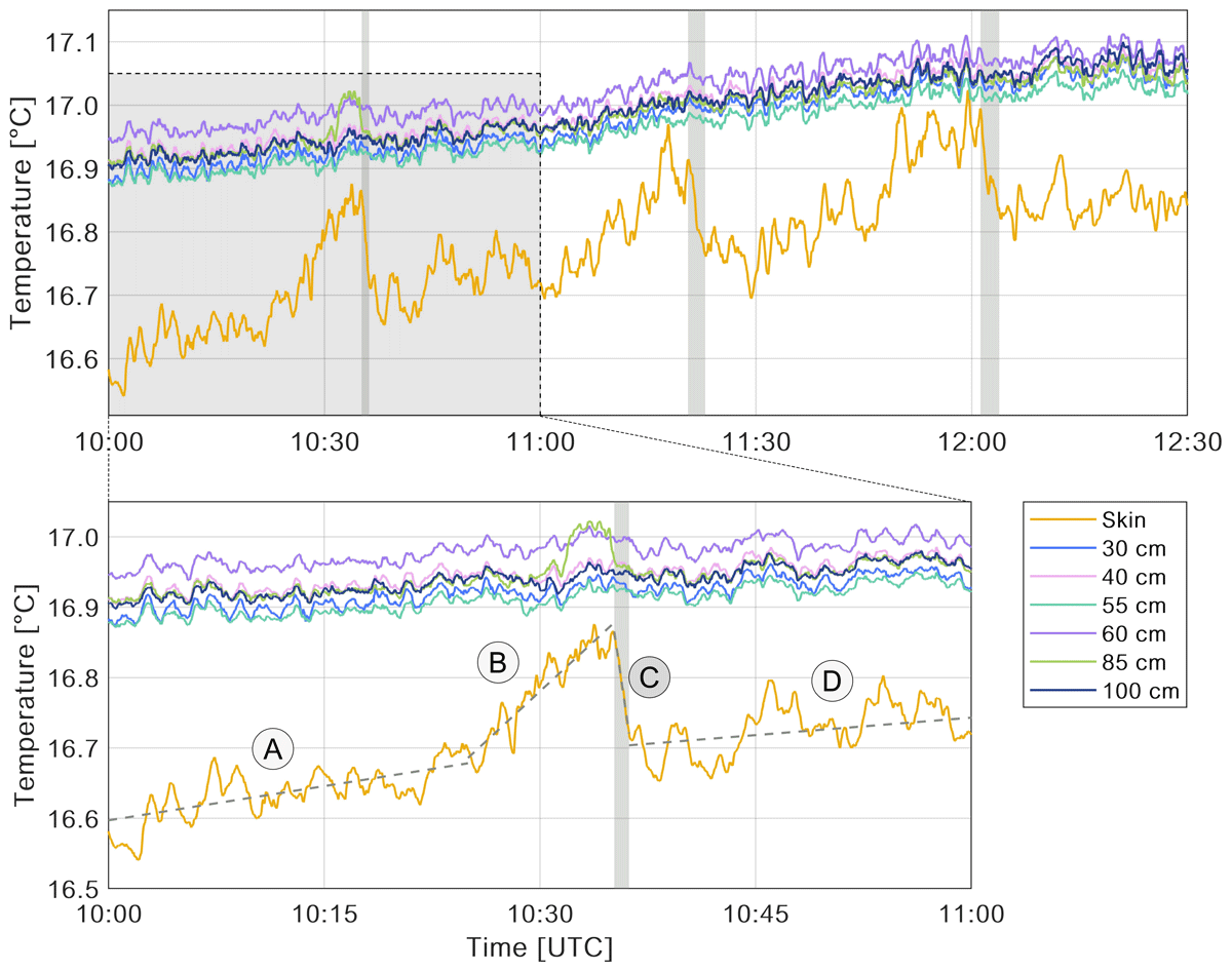
Figure 1
Time series of temperature in the skin and near-surface layer at various depths during three artificial disturbances of the ocean’s surface (top) and zoomed time series of the first disturbance (bottom). Dashed lines are temperature regression lines of the skin layer for phases: (A) before disturbance, (B) during disturbance, (C) recovery of the thermal skin layer, and (D) after recovery. Gray bars represent the duration of thermal skin recovery. (Zoomed time series for disturbances two and three see Figure S3.)
The ADCP recorded current velocities starting at a depth of 2.6 m and extended downward through the water column. At this depth, measurements averaged over a 10-minute interval during the recovery process yielded 0.39 ± 0.14 m s–1, 0.38 ± 0.14 m s–1, and 0.32 ± 0.10 m s–1, for each disturbance respectively. In comparison, maximum mean current velocities in the German Bight reached 0.49 m s–1 (Deyle et al. 2024) and those in the northern North Sea reached 0.67 m s–1 (Vindenes et al. 2018). These results highlight the presence of moderately strong tidal currents, which contributed to the mixing of surface waters and counteracting the formation of stratification.
During the disturbances, Tskin closely approached the temperatures of the near-surface layer, with a deviation of 0.083 ± 0.022°C just before the recovery. The discrepancy is likely due to ongoing upward heat fluxes, as the skin temperature does not fully equilibrate with the underlying water, even under conditions of high wind and turbulent mixing (Castro, Wick and Emery 2003; Wells et al. 2009). For each disturbance, Tskin revealed four distinct phases (Figure 1, bottom panel). Initially (phase A), a minor increase in temperature was noted, which was attributed to diurnal warming followed by a stronger temperature increase due to artificial mixing with the warmer underlying water (phase B). Subsequently, the skin layer underwent a recovery phase (phase C) and gradually returned to its cooler state. Finally, post-thermal recovery (phase D) followed and merged with phase A of the next disturbance. The recovery times were 62 s, 144 s, and 157 s (Table 1), respectively. From the first to the last recovery, the skin temperature difference during the recovery increased from 0.140 to 0.162°C.
Table 1
Time of the onset of the recovery phase, skin layer recovery times (t*), skin temperatures before (Tskin start) and after recovery (Tskin end), skin temperature difference (Tskin diff), and temperature anomalies before and after recovery (ΔT = Tskin – T100 cm) for each of the three disturbances.
| TIME UTC [hh:mm:ss] | t* [s] | Tskin START [°C] | Tskin END [°C] | Tskin DIFF [°C] | ΔT START [°C] | ΔT END [°C] | |
|---|---|---|---|---|---|---|---|
| 1st Disturbance | 10:35:10 | 62 | 16.861 | 16.721 | 0.140 | –0.086 | –0.229 |
| 2nd Disturbance | 11:20:32 | 144 | 16.914 | 16.764 | 0.150 | –0.103 | –0.248 |
| 3rd Disturbance | 12:01:12 | 157 | 16.995 | 16.833 | 0.162 | –0.060 | –0.217 |
We performed linear regression for each of the four phases, and the recovery rates were –0.140°C min–1, –0.070°C min–1, and –0.047°C min–1 for the first, second, and third disturbance, respectively (Table 2), hence slowing down by a factor of approximately three from the first to the last disturbance.
Table 2
Temperature rates in °C min–1 for phase A-D which are shown as regression lines in Figure 1 and Figure S3. The recovery rates (Rt) of the cool-skin layer are highlighted in bold.
| BEFORE (A) | DISTURBANCE (B) | RECOVERY (C) | AFTER (D) | |
|---|---|---|---|---|
| 1st Disturbance | 0.003 | 0.019 | –0.140 | 0.002 |
| 2nd Disturbance | 0.002 | 0.013 | –0.070 | 0.003 |
| 3rd Disturbance | 0.003 | 0.052 | –0.047 | 0.000 |
During the experiment, the average air temperature was 15.0 ± 0.2°C and increased by 0.5°C during the observations (Figure 2). Averaged wind speeds (over three minutes) during the first, second, and third disturbance were 4.75 ± 0.35 m s–1, 4.40 ± 0.36 m s–1, and 3.96 ± 0.84 m s–1, respectively. The averaged evaporation rate was 0.13 ± 0.02 mm h–1, and decreased by 0.01 mm h–2 with decreasing wind speed during the experiment (Figure S4). The increasing temperature in the skin and near-surface layer (Figure 1) indicates diurnal warming with a rate of 0.003°C min–1 prior to the first disturbance, but which leveled off after the third disturbance (Table 2).
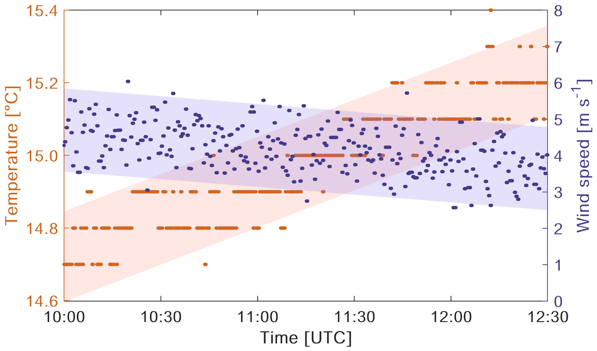
Figure 2
Air temperature (red) and wind speed (blue) recorded during the experiment by the autonomous surface vehicle Halobates. The shaded area represents a 95% prediction interval for the estimated regression lines.
The overall positive and increasing net air-sea heat flux (QN) throughout the day was primarily driven by the shortwave heat flux, which reflected the solar radiation reaching its daily maximum at 12:10 UTC (Figure 3). In contrast, the sensible, latent, and longwave heat fluxes were negative, thus cooling the sea surface. With increasing air temperature and decreasing wind speed, the sensible and latent heat fluxes decreased by 26% and 14%, respectively (Figure 3). Most of the heat was lost through the longwave radiation emitted by the sea surface at a constant rate throughout the experiment. Based on Equation 3, we calculated the net air-sea heat flux specifically for the upper millimeter of the ocean (QN skin). Within the skin layer, QN skin was negative, averaging –135 W m–2 and decreased by 26% over time (Figure 3). QN skin had an estimated uncertainty of ±17 W m–2, calculated by error propagation through all heat flux components.
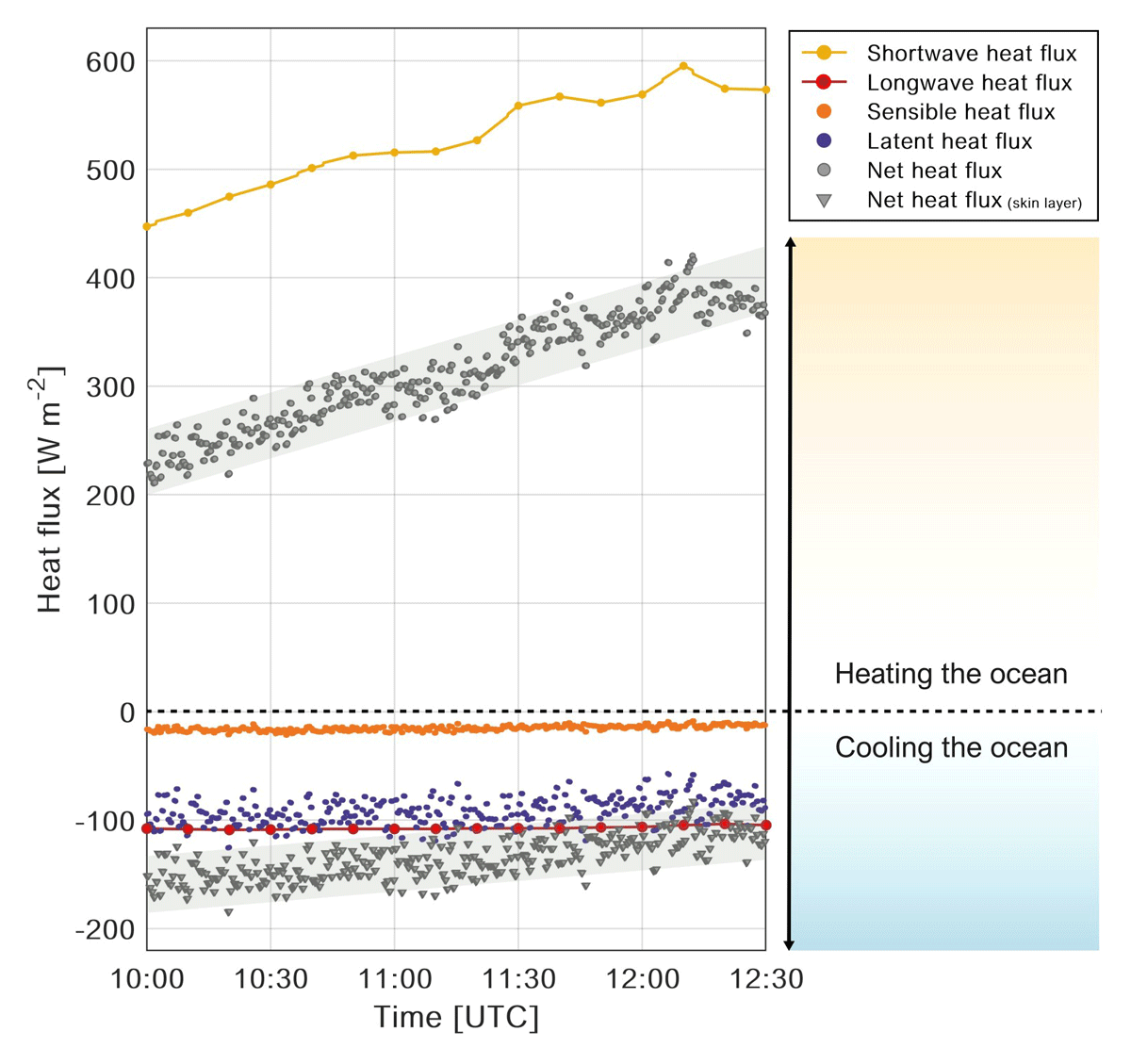
Figure 3
Components of the air-sea heat flux: Shortwave heat flux (yellow line) calculated based on measurements of incoming shortwave radiation (yellow dots). Longwave heat flux (red line) calculated based on measurements of downwelling and upwelling longwave radiation (red dots). Sensible (orange) and latent heat flux (blue) calculated using the COARE 3.6 algorithm (Fairall et al. 2003). Gray dots represent net air-sea heat flux, while gray triangles represent the net heat flux of the skin layer (approx. 1 mm). The shaded area represents a 95% prediction interval for the estimated regression lines.
Using the skin layer heat flux (QN skin) and the recovery times (t*) for each disturbance, the theoretical recovery change temperatures ΔTτ, a measure of possible temperature change during recovery, were calculated as 0.85°C, 1.16°C and 1.09°C (Table 3), substantially exceeding the observed temperature changes. QN skin and ΔT were used to calculate the scaling depths δ representing the thickness of the thermal boundary layer that was 1.06 ± 0.16 mm during times of no disturbance (Figure 4). The uncertainty in scaling depths, propagated from heat flux budget errors, is ± 0.12 mm. During all three disturbances, the thickness approached 0.2 mm, indicating a significant reduction in the thermal boundary layer due to enhanced turbulence from the artificial mixing. However, a thin boundary layer remained. The typical thickness of the skin layer δ was used together with the temperature recovery rates Rt to calculate the restoring internal energy flux which decreased from the first to the third experiment from 10.15 to 3.41 W m–2 (Table 3).
Table 3
Net heat flux in the skin layer QN skin, recovery temperature change ΔTτ for recovery times t*, and the restoring internal energy flux Jr for each of the three disturbances.
| QN skin [W m–2] | ΔTτ(t*) [°C] | Jr [W m–2] | |
|---|---|---|---|
| 1st Disturbance | –147.61 | 0.846 | 10.15 |
| 2nd Disturbance | –132.58 | 1.158 | 5.07 |
| 3rd Disturbance | –119.19 | 1.087 | 3.41 |
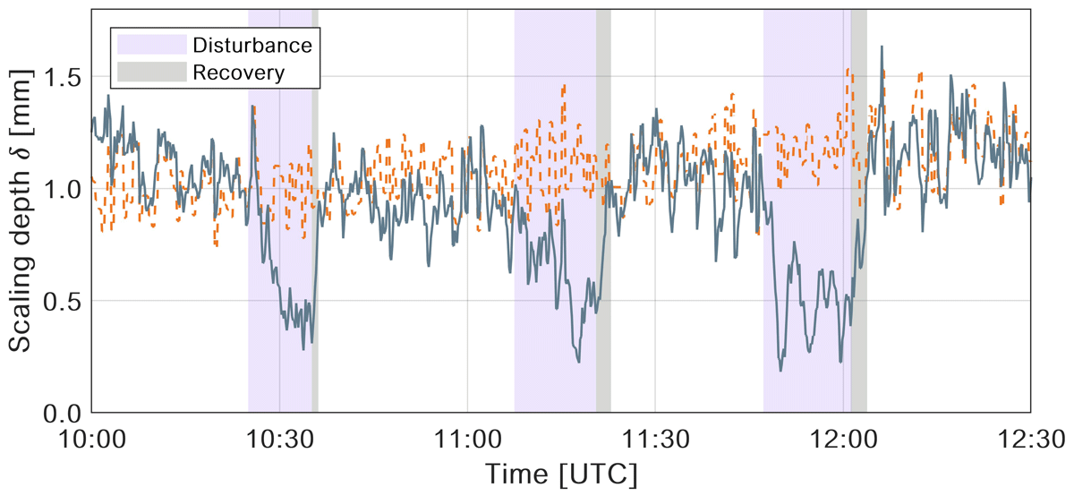
Figure 4
Comparison between the calculated scaling depths of the thermal skin layer from a bulk formula by Katsaros (1980) (blue line) and the thickness of the skin layer calculated with the COARE 3.6 algorithm (dashed orange line). Shaded areas indicate periods of artificial disturbance and the subsequent recovery.
4 Discussion
We have described a new approach for measuring skin layer recovery after artificial disturbances under natural conditions. Based on the outboard engine horse power, half of full speed, and a comparative analysis by Nedohin and Elefsiniotis (1997), we estimate vertical mixing of more than three meters. This vertical mixing ensured that the skin layer and the near-surface layer were thoroughly mixed before the recovery phase. As confirmed by the temperature measurements at various depths (Figure 1) the near-surface layer was well-mixed throughout the observation, due to strong tidal currents in the study area (Otto et al. 1990; Wurl et al. 2024). The experiments allowed us to detect the maximum values of t* under the prevailing wind and heat flux conditions.
The wind and heat flux conditions changed from the first to the last artificial disturbance, leading to changes in the recovery process of the cool-skin layer. The opposing effects of wind-driven turbulent mixing and solar absorption are the main drivers that cause diurnal variabilities in sea-surface temperature and, thus, skin layer temperature anomalies (Börner, Haerter and Fiévet 2024). A decrease in wind speed reduces evaporation fluxes (Singh and Xu 1997), which was reflected in the decline of latent heat flux. Additionally, as the wind speed decreased and the air temperature increased, the sensible heat flux decreased over the course of the observation (Large and Pond 1982). An increase in solar radiation throughout the day further reduced the net heat flux in the skin layer. The recovery times for the cool-skin layer progressively increased from 64 seconds in the first disturbance to 144 seconds in the second and 157 seconds in the third. This progression underscores the critical role of heat flux in the recovery process, with a decreasing net heat flux in the skin layer contributing to longer recovery times (t*). Additionally, the restoring internal energy flux (Jr), which represents the upward transfer of heat within the water column, decreased over the course of the experiments due to decreasing recovery rates (Rt) (Tables 2 and 3). With reduced internal energy fluxes, the capacity of the cool-skin layer to restore thermal equilibrium after a disturbance was weakened, thereby requiring longer recovery phases.
Zappa, Jessup and Yeh (1998) reported that patches of artificially induced disturbances did not fully recover within up to 80 seconds before drifting out of the infrared camera’s field of view. It was shown that disturbances with higher wave Reynolds numbers produced larger wakes, which took more time to fully recover. Zappa, Jessup and Yeh (1998) extrapolated their observations and estimated recovery times of 120 seconds. Two of our recovery times exceeded Zappa et al.’s estimate by 24 and 37 seconds. Our measurements indicate that under conditions of complete mixing, typically associated with a higher wave Reynolds number, recovery times (t*) can extend up to three minutes or even longer, depending on the net surface heat flux within the skin layer. Conversely, disturbances with lower wave Reynolds numbers, such as those resulting from small-scale wave-breaking events, tend to recover much more rapidly, typically within a few seconds (Ewing and McAlister 1960; Jessup et al. 1997).
The theoretical recovery change temperatures (ΔTτ), derived from the recovery time t* of each disturbance, exceeded the actual observed temperature change by 0.88 ± 0.13°C (Table 3). This discrepancy suggests that the heat transfer processes may be more complex than those accounted for in the model proposed by Jessup et al. (2009). The model likely overestimates the recovery rate, because the actual process may be slower due to more gradual heat redistribution. Corresponding to Donlon et al. (1999), when wind speed exceeds 3 to 4 m s–1 shear-driven turbulent heat-transfer dominates over molecular and convective heat transfer (Veron and Melville 2001). In our experiments, surface turbulent mixing from the slow decay of the induced disturbance, tidal currents (Otto et al. 1990), or wind-enhanced currents (Zhang and Chen 2023), likely contributed to the observed recovery dynamics, explaining the overestimation in ΔTτ.
During periods of no disturbance, the range of the calculated thickness of the thermal skin layer closely matched the cool-skin thickness computed by the COARE 3.6 algorithm (Figure 4), suggesting that, in this case, the bulk formula aligns well with the algorithm with precise parameterizations. With an average thickness of 1.06 ± 0.16 mm these findings are consistent with typical scaling depths under undisturbed conditions (Schimpf, Garbe and Jähne 2004; Wells et al. 2009). However, when turbulent mixing is introduced, as noted by Wells et al. (2009), the thickness of the thermal boundary layer decreases. This is because turbulent mixing enhances the convective transfer of heat, effectively reducing the temperature gradient near the surface and resulting in a thinner boundary layer. Consistent with this, our findings show that during periods of disturbance, the thermal boundary layer thickness decreased to approximately 0.2 mm before gradually increasing again during the recovery phase. To further enhance the COARE 3.6 algorithm, an option to input both skin and bulk temperatures could be introduced, allowing for greater accuracy in cases where both measurements are available.
5 Conclusions
In this study, we present a novel approach to quantify ocean skin temperature anomalies under the influence of complete artificial disturbances of the near-surface layer. During the disturbances, the previously existing cool-skin layer dissipated, thereby reducing the thickness of the thermal boundary layer. Subsequently, the recovery of the cool-skin layer was observed under natural conditions. Finally, we tested Zappa, Jessup and Yeh’s (1998) hypothesis that cool-skin recovery can take up to 120 seconds, and extended this by showing that recovery times can be even longer, depending on the surface heat flux within the skin layer. It was demonstrated that complete thermal recovery can take up to three minutes, which is significantly longer than the recovery times typically observed for less disruptive events, which can recover in just a few seconds (Jessup et al., 1997). Our investigation focused on the conditions of complete mixing within the surface layer, providing deeper insight into the recovery dynamics under more energetic perturbations.
Data Accessibility Statement
Data and metadata generated and analyzed during this study are available in the PANGAEA data repository (https://doi.org/10.1594/PANGAEA.968959, Jaeger et al. (2024)).
Additional File
The additional file for this article can be found as follows:
Acknowledgements
We sincerely thank the crew and scientists aboard the RV Senckenberg for their time and efforts in the deployment of Halobates during the cruise. Further, we thank Thomas Badewien, Jens Meyerjürgens and Lisa Deyle from the group Marine Sensor Systems at the Institute for Chemistry and Biology of the Marine Environment (ICBM) for providing ADCP data from the joint field campaign.
Competing Interests
The authors have no competing interests to declare.
Author Contributions
O.W. and L.G. conceived and conducted the field survey. S.M.A. compiled the dataset. L.J. completed the data compilation and conducted data analysis with assistance from R.B. L.J. made the figures and drafted the manuscript with support from O.W. All authors discussed and finalized the manuscript.