
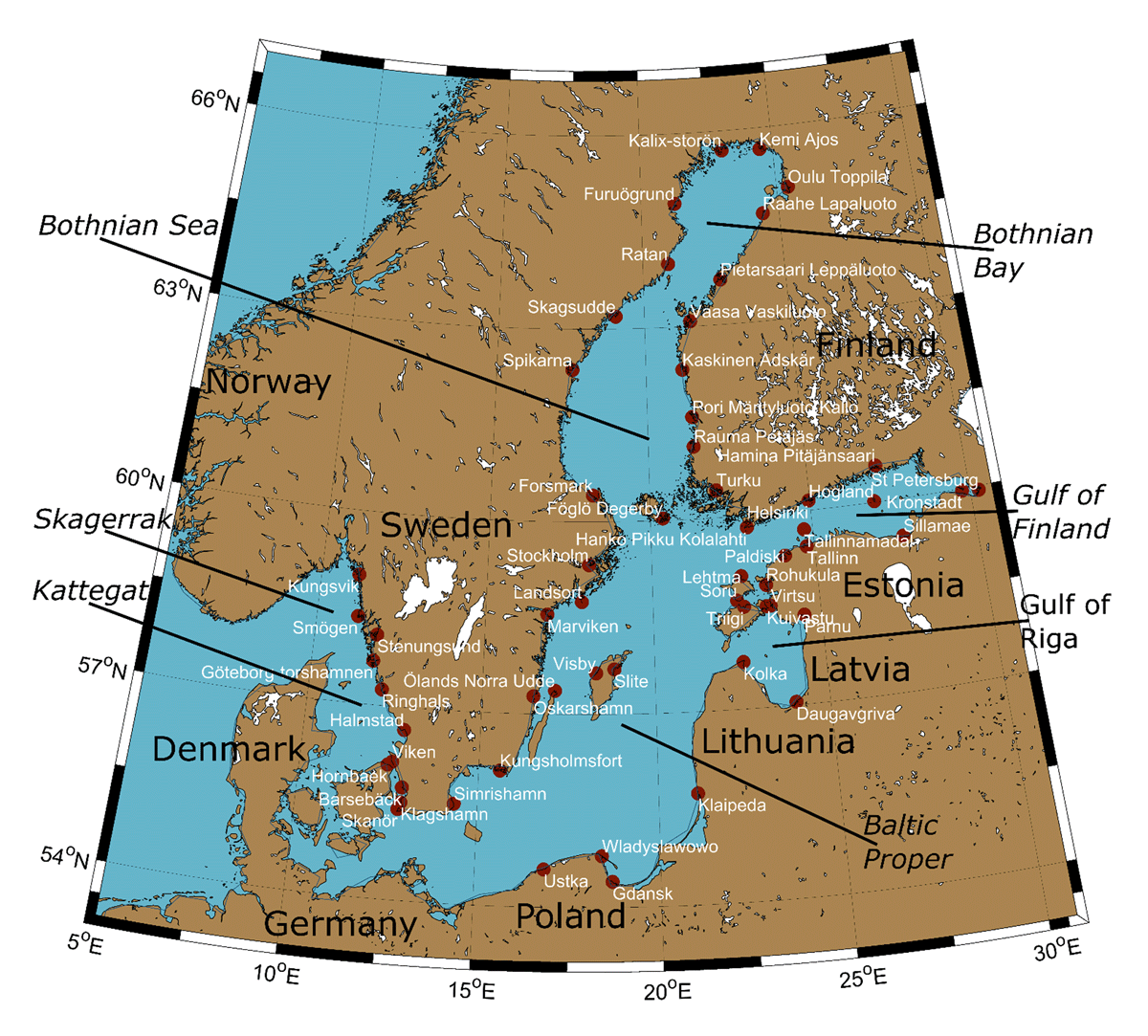
Figure 1
Regional map of Northern Europe showing sea level stations (in white text) of interest (Pawlowicz, 2020), with the Baltic Sea and its basins (in italic) based on Klemeshev et al. (2017) and Weisse et al. (2021).
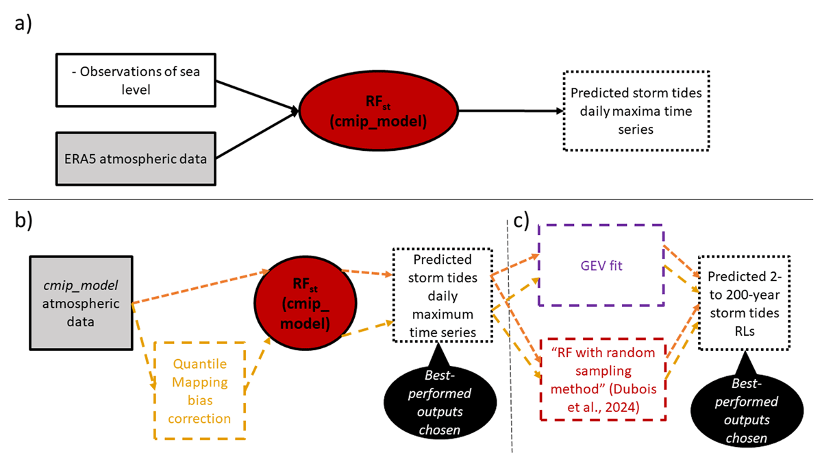
Figure 2
Workflow illustrating the methodology used in this study, applied at each site (“st”) and for each CMIP model independently. The model RFst(cmip_model) (in red bubble) is trained using sea level observations and ERA5 reanalysis atmospheric data (panel a). Atmospheric data from each CMIP model is used either directly as input or processed through a quantile-mapping bias correction method before being input into RFst(cmip_model) to predict daily maximum storm tide time series from 1850 to 2100 at the site “st” for each CMIP model (panel b). Predicted daily time series are then analysed through a GEV fit and an “RF with random sampling” method to obtain 2- to 200-year storm tide return levels (RLs), allowing for analysis of extreme storm tides (panel c). The best-performing outputs from the daily time series and predicted RLs are selected for results analysis based on RMSE values. Solid rectangles represent datasets, with grey rectangles indicating atmospheric datasets. Predictions are highlighted in dashed black rectangles, while methods are highlighted in coloured dashed rectangles. Yellow denotes climate input datasets that underwent quantile mapping bias correction, while orange indicates the ones that did not.
Table 1
Summary of climate models used.
| MODEL (CMIP_MODEL) | EC-EARTH3 (EC-EARTH) | IPSL-CM6 A-LR (IPSL) | MPI-ESM1.2-LR (MPI_LR) | GFDL_ESM4 (GFDL_ESM4) |
|---|---|---|---|---|
| Institution | EC-Earth Consortium | Institut Pierre-Simon Laplace (France) | Max Planck Institute for Meteorology (Germany), also Deutsches Klimarechenzentrum (Germany) and Deutscher Wetterdienst (Germany) | NOAA-Geophysical Fluid Dynamics Laboratory (USA) |
| Model reference and dataset DOIs | Döscher et al. (2022) https://doi.org/10.22033/ESGF/CMIP6.251 | Boucher et al. (2020), Hourdin et al. (2020), Lurton et al. (2020) https://doi.org/10.22033/ESGF/CMIP6.1532 | Mauritsen et al. (2019) https://doi.org/10.22033/ESGF/CMIP6.793 | Dunne et al. (2020) https://doi.org/10.22033/ESGF/CMIP6.1414 |
| Approximate spatial resolution (degrees) | 0.75 * 0.75 | 2.5 * 1.25 | 1.875 * 1.875 | 1 * 1 |
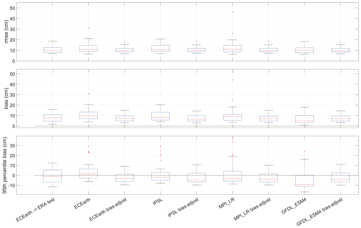
Figure 3
GOF metrics over the daily maxima time series of each RF model with three inputs (ERA, CMIP6, and CMIP6 bias adjusted) for the four climate models at each station. GOF metrics are calculated from the sorted scatter plots. ERA5 statistical coefficients are measured based on the testing period whereas CMIP6 and CMIP6 bias-adjusted statistical coefficients are based on the validation period (Table A1).
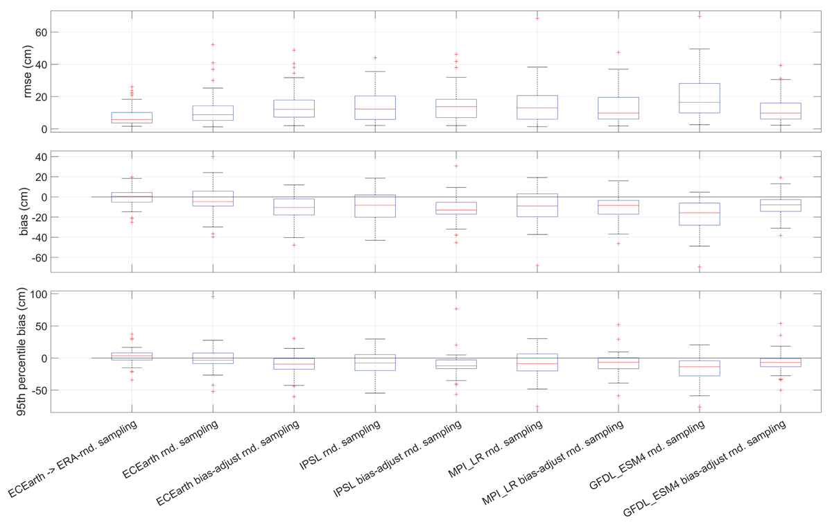
Figure 4
GOF metrics over the storm tide RLs of each RF model with three inputs (ERA, CMIP6, and CMIP6 bias adjusted) for the four climate models at each station where the GEV fit converges. GOF metrics are calculated from the sorted scatter plots for both the mean predictions and the RF method with random sampling (Dubois et al., 2024). ERA5 statistical coefficients are measured based on the testing period whereas CMIP6 and CMIP6 bias-adjusted statistical coefficients are based on the validation period (Table A1).
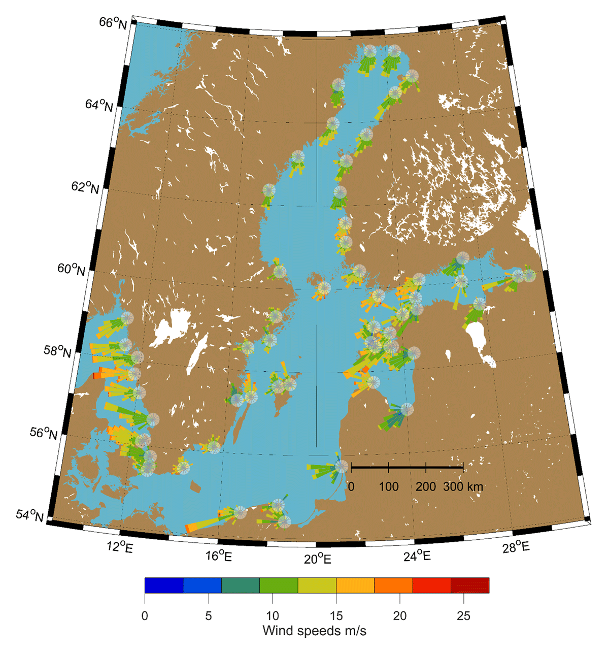
Figure 5
Characteristics of wind direction and wind speed (wind roses) from ERA5 reanalysis associated with ESL events defined as independent events with daily maxima sea level above the 95th percentile threshold value obtained from observation time series at each station over the co-occurring period (Table. A1).
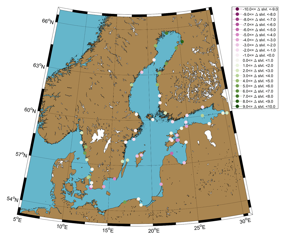
Figure 6
Difference values of the ensemble mean from the four climate models of the 50-year RL storm tide calculated between the 2070–2099 and 1850–1879 periods at each station (cf. section 2.2.3).
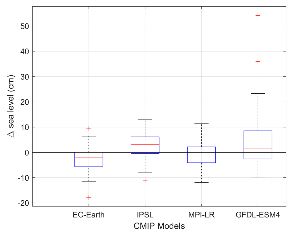
Figure 7
Box plots of the difference in 50-year RL storm tide between 2070–2099 and 1850–1879 at each station, grouped by climate model.
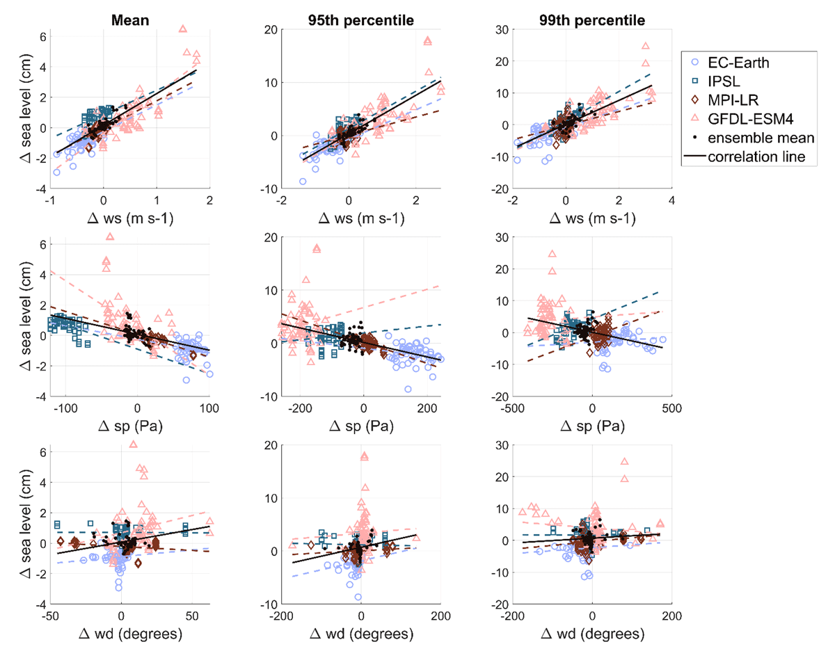
Figure 8
Scatter plots of the difference values of the mean, 95th and 99th percentiles (for each column) from the atmospheric variables: wind speed (ws), wind direction (wd), and the 5th and 1st percentiles of surface pressure (sp) (x-axes) against sea level (y-axes), calculated between 2070–2099 and 1850–1879 at each station, and for each climate model, as well as for the ensemble mean.
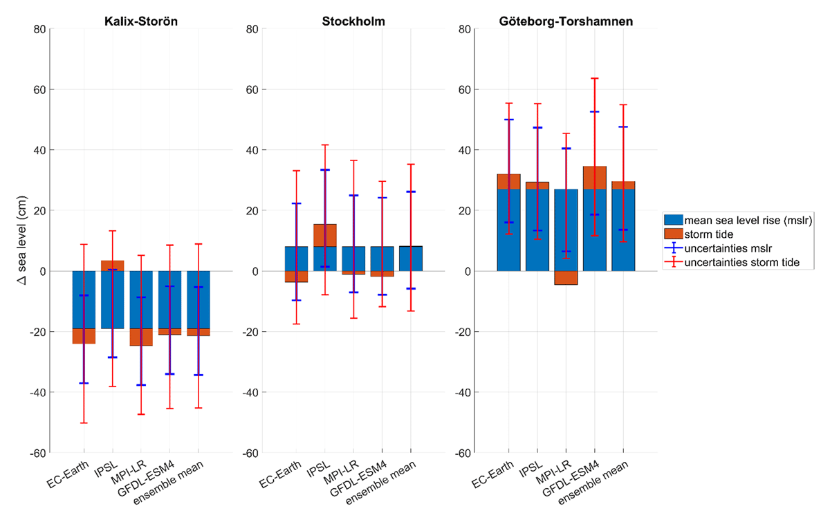
Figure 9
Difference values of the 50-year RL storm tide calculated between the 2065–2094 and 1985–2014 periods displayed with projected local mean sea level changes by 2080 under SSP2–4.5 (SMHI, 2020) at stations Kalix, Stockholm, and Göteborg. Uncertainties associated with each projection are shown as error bars (95th percentile confidence interval) centred on the cumulative total sea level.