
1. Introduction
Coastal floods impact coastal ecosystems and our societies by disrupting human activities on the coast, resulting in considerable economic losses and community disruptions, often leading to fatalities (EEA, 2024; IPCC, 2023; Vousdoukas et al., 2020; Wahl et al., 2017). Economic losses due to coastal floods have been projected to increase by orders of magnitude by 2100 compared to today in Europe if no urgent actions are taken to mitigate impacts in vulnerable areas (Vousdoukas et al., 2018). The North Sea and the Baltic Sea are areas prone to coastal floods (Halsnæs et al., 2016; Rutgersson et al., 2022).
Extreme sea levels (ESLs) are caused by multiple factors, such as tides, waves, winds, bathymetry, and terrain features, but also by river runoff and precipitation during compound coastal flood events. In a changing climate, the frequency and severity of extreme events are expected to change in the future, increasing risks from natural hazards including coastal floods (Rutgersson et al., 2022; Seneviratne et al., 2021). At the global scale, the sea level is rising due to climate change and this rise is accelerating (Church et al., 2013; Dangendorf et al., 2019) but with regional differences (Fox-Kemper et al., 2021; Melet et al., 2024; Vousdoukas et al., 2017), including in the Baltic Sea, which is projected to be around 87% of the global rise (Meier et al., 2022a). Relative sea level rise is found to be the main driver of future changes in ESLs in Europe (Abadie et al., 2019; IPCC, 2022; Paprotny and Terefenko, 2017). However, in Northern Europe, the influence of changes in extratropical cyclones on ESLs is projected to be more significant (Vousdoukas et al., 2018), especially in the Kattegat and Baltic Sea (Vousdoukas et al., 2016), regions with complex geometries (Andrée et al., 2021) where relative sea level rise is regionally balanced by land uplift due to post-glacial rebound (Hieronymus and Kalén, 2020; Pellikka et al., 2023). Meier et al. (2022a) highlight that ESLs over the Baltic Sea depend on wind velocities and storm tracks, which do not show systematic changes in the future according to Christensen et al. (2022), but with very high uncertainty (Meier et al., 2022b). Changes in storm surges are therefore not expected and are associated with a low confidence level, which necessitates further research (Rutgersson et al., 2022). Hence, it is relevant to consider future changes in storm surges, and not only relative sea level rise, in this area when projecting coastal flood hazards.
All of these processes are important to consider for providing reliable estimates of ESLs on different timescales, which are essential for coastal management and spatial planning to mitigate a potentially higher risk of coastal floods in the Baltic Sea (Halsnæs et al., 2023; Hieronymus and Kalén, 2022; Su et al., 2021; Van de Wal et al., 2023). This requires robust multi-decadal predictions and century-long projections of oceanographic, atmospheric, and hydrologic conditions. Such information generally derives from global circulation and Earth System Models. These computationally expensive dynamical models have a resolution that is too coarse to accurately predict local extreme events and they are associated with relatively high uncertainties (Hawkins and Sutton, 2009). For example, predicting storm surges requires higher spatial and temporal resolution to accurately model hydrodynamic processes in near-shore waters compared with atmospheric storms (Stanev et al., 2016), which current global climate models fail to reproduce at these fine scales. Regional climate models based on dynamic downscaling (Pätsch et al., 2017; Tapiador et al., 2020) and empirical-statistical downscaling techniques (Gebrechorkos et al., 2023; Jimenez et al., 2024; Vaittinada Ayar et al., 2016) have been introduced to address this issue. Methodologies have therefore been developed to predict coastal oceanographic conditions, such as ESLs, for the next century, considering the current changing climate. Woth et al. (2005) predicted storm surges around the North Sea for the period 2070–2100 based on dynamical modelling using four regional climate models as atmospheric forcing. Gaslikova et al. (2013) also dynamically modelled storm surges for the North Sea based on four different future scenarios from 1960 to 2100. Muis et al. (2020) developed a framework based on high-resolution dynamic models to project storm tides and ESLs globally until 2050. Krieger et al. (2024) demonstrated the possibility of using machine learning neural networks to predict storm surges at Cuxhaven (Germany) on decadal time scales based on mean sea-level pressure fields. Kaufmann et al. (2024) used neural networks to predict the impact of climate change on storm surges until 2060 in Southeast Brazil. Ayyad et al. (2023) predicted hurricane storm surges for the New York/New Jersey coastlines from 1980–2100 using the Adaptive Boost algorithm with support vector regressor machine learning models.
The main goal of the current study was to investigate characteristics and changes in storm tide hazard at the local scale around the Baltic Sea (Figure 1) from 1850 to 2100. We started by briefly analysing atmospheric conditions leading to ESLs at 59 different stations around the Baltic Sea. We then explored the potential changes in storm tides driven by atmospheric variability by the end of this century and later related these changes to the context of climate change, associated with regional relative sea level rise. To achieve this, a random forest (RF) machine learning model was trained using observations of tide gauges at each station and local atmospheric drivers from reanalysis datasets at each site independently. Next, atmospheric variables extracted from four different climate models in the 250-year period of 1850–2100, based on the medium-emission scenario SSP2–4.5 (O’Neill et al., 2016), were used as inputs to our RF model, resulting in a small ensemble of daily maxima time series of sea levels. From these runs, differences between future and historical storm tides were analysed and linked with changes in atmospheric conditions.
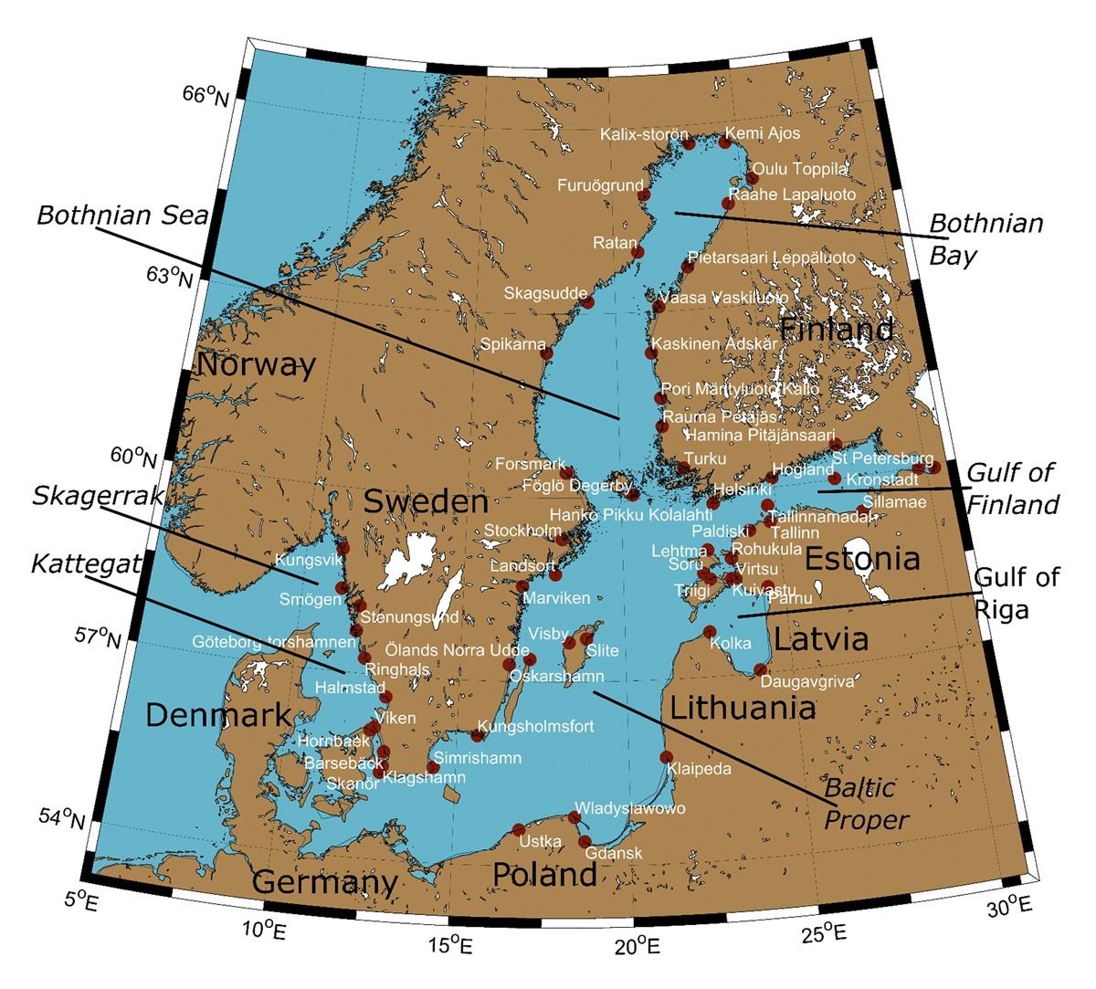
Figure 1
Regional map of Northern Europe showing sea level stations (in white text) of interest (Pawlowicz, 2020), with the Baltic Sea and its basins (in italic) based on Klemeshev et al. (2017) and Weisse et al. (2021).
2. Data and Methods
In the following, we analyse ESLs primarily related to storm tides, defined as the sea level height resulting from the combination of storm surges and tides. This focus is motivated by the low tidal range of only a few centimetres in the Baltic Sea, and of approximately 40 cm and 20 cm during spring tides in the Skagerrak and Kattegat basins, respectively (Klemeshev et al., 2017; Medvedev et al., 2013; Weisse et al., 2021).
The main steps of the workflow representing the employed methodology are presented in Figure 2 and explained further in section 2.2. The RF machine learning method is used to predict storm tides at various stations based on sea level observations and on atmospheric variables from reanalysis and hindcast datasets (Figure 2a), as well as climate models (Figure 2b). The observations are used during training and also for evaluation purposes. The atmospheric variables are the inputs used by the RF models to predict storm tides. Tadesse et al. (2020) successfully showed that data-driven models (linear regression and RF) can predict daily maximum storm surges based on mean sea level pressure and wind speeds from reanalysis datasets at the global scale. Bellinghausen at al. (2025) successfully used RF to predict the occurrence of ESLs based on atmospheric variables (surface pressure, zonal, and meridional wind speeds, and precipitation) at the Baltic Coast with lead times of up to three days. These predictions are here later combined with local relative mean sea level changes, driven by mean sea level rise due to climate change and Glacial Isostatic Adjustment, to estimate the total ESL.
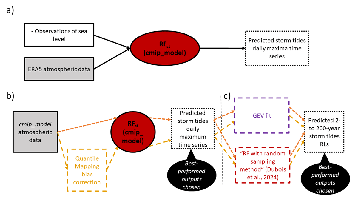
Figure 2
Workflow illustrating the methodology used in this study, applied at each site (“st”) and for each CMIP model independently. The model RFst(cmip_model) (in red bubble) is trained using sea level observations and ERA5 reanalysis atmospheric data (panel a). Atmospheric data from each CMIP model is used either directly as input or processed through a quantile-mapping bias correction method before being input into RFst(cmip_model) to predict daily maximum storm tide time series from 1850 to 2100 at the site “st” for each CMIP model (panel b). Predicted daily time series are then analysed through a GEV fit and an “RF with random sampling” method to obtain 2- to 200-year storm tide return levels (RLs), allowing for analysis of extreme storm tides (panel c). The best-performing outputs from the daily time series and predicted RLs are selected for results analysis based on RMSE values. Solid rectangles represent datasets, with grey rectangles indicating atmospheric datasets. Predictions are highlighted in dashed black rectangles, while methods are highlighted in coloured dashed rectangles. Yellow denotes climate input datasets that underwent quantile mapping bias correction, while orange indicates the ones that did not.
2.1 Data
2.1.1 Sea level data
In this study, sea level observations with an hourly timestep were used. These observations were obtained from 59 stations (Figure 1), available from the Swedish Meteorological and Hydrological Institute (SMHI), the Swedish Maritime Administration (Sjöfartsverket), the Danish Meteorological Institute (DMI), the Finnish Meteorological Institute (FMI), and the Global Extreme Sea Level Analysis (GESLA) v3 dataset (Haigh et al., 2022). The time series vary in length, spanning from seven to more than 100 years (Table A1). Stations with shorter time periods on record present higher uncertainties when analysing ESLs due to the scarcity of such rare events.
Datasets with higher temporal resolution are averaged into hourly mean time series. Each dataset is then linearly detrended and transformed from hourly to daily maxima time series before being used for the analysis. As each dataset is not de-tided due to the previously mentioned low tidal range, we therefore refer to storm tides rather than storm surges. ESLs are further investigated as storm tides annual maxima values or storm tides values above a defined threshold (95th or 99th percentiles), with a minimum temporal separation of two days, to ensure independence between each event.
2.1.2 Atmospheric data
Meteorological data (wind speed, wind direction, and surface pressure) are the key drivers of storm tides and were therefore used as input datasets for the machine learning models. The variables downloaded for this study include the eastward and northward components of the wind at 10 meters height, and surface pressure. Time-consistent reanalysis datasets are primarily relevant for training each RF model alongside sea level observations, while climate datasets are important for projecting storm tides through the end of the century.
- ERA5 reanalysis
The ERA5 global and hindcast reanalysis dataset (ERA5) provides atmospheric, oceanographic, and land information from 1940 to 2023, with a spatial resolution of 31 km and hourly temporal resolution (Hersbach et al., 2023). ERA5 is used to analyse the atmospheric drivers of ESLs at each station, based on the closest sea-based grid point (section 2.2.1). To train the RF model for projecting storm tides (section 2.2.2), ERA5 data is also obtained from the nearest sea-based grid point corresponding to each cmip_model closest sea-based grid point for each station. To match the 3-hourly temporal resolution from the climate models, ERA5 hourly time series are averaged into 3-hourly mean time series.
- CMIP6 projections
Climate atmospheric datasets from the Coupled Model Intercomparison Project Phase 6 (CMIP6) (O’Neill et al., 2016) were obtained for four global models with 3-hourly temporal resolution, covering both historical periods (1850 to 2015) and future projections (2015 to 2100) under the SSP2–4.5 scenario: EC-Earth, IPSL, MPI_LR, and GFDL_ESM4. We named the variable cmip_model to refer to any of these climate model independently. The spatial resolutions differ between models. These models were selected as they were the only CMIP6 models with 3-hourly temporal resolution available for both the historical period and SSP2–4.5 climate scenario from the Earth System Grid Federation (ESGF) data node (https://aims2.llnl.gov/search) at the time of download. For each model, data from the closest sea-based grid point was obtained at each station.
2.2 Methods
The approach for analysing ESLs around the Baltic Sea at the local scale of each station was based on projecting storm tides using the RF model (Breiman, 2001) for each station individually. First, an analysis of the current atmospheric drivers of ESL was conducted at each station to better understand the local atmospheric conditions leading to ESL (section 2.2.1). Then, a probabilistic RF model was trained with sea level observations and ERA5 datasets for each station and for each cmip_model independently and was denoted RFst(cmip_model) (Figure 2a). RFst(cmip_model) was used to project daily maximum sea level time series from 1850 to 2100, forced with the respective CMIP6 climate model dataset for each station (Figure 2b) (section 2.2.2). Next, the generalized extreme value (GEV) distribution (Coles, 2001) and the RF with random sampling method (Dubois et al., 2024) was applied to analyse return levels (RLs) of storm tides at each station (Figure 2c) (section 2.2.3). Finally, the total sea level RLs were obtained by adding the local relative sea level rise to the projected storm tide time series.
2.2.1 Atmospheric Characteristics of ESL
Local variations in oceanographic, atmospheric, and topographic conditions at stations around the Baltic Sea may result in distinct ESL characteristics, reflecting site-specific natural drivers. To obtain a deeper understanding of the atmospheric conditions that lead to storm tides, each site was analysed based on its sea level observations and the ERA5 meteorological datasets.
For each station, the dates of ESL events were obtained when the sea level reached its annual maxima (first set) and when the sea level values were above the 95th (second set) and 99th (third set) percentiles threshold values calculated over the sea level daily maxima time series. To ensure the independence of storm events, a minimum temporal separation of two days between each event was enforced. The corresponding daily values of minimum surface pressure, maximum wind speed and corresponding wind direction were extracted from the ERA5 dataset at the closest sea-based grid point indicating the meteorological drivers of storm tides at each site.
2.2.2 Model: Sea level daily maxima time series
Following the general methodology (Figure 2), RFst(cmip_model) used the atmospheric variables: wind speed, wind direction, surface pressure, and the month of the year as inputs. RFst(cmip_model) was trained using ERA5 datasets (Figure 2a) and applied with CMIP6 model datasets for future projections (Figure 2b). The closest grid point over sea from each CMIP6 model used was extracted for each station and referred to as CMIP6st(cmip_model). The nearest ERA5 sea-based grid point to CMIP6st(cmip_model) was used to train the model. This approach ensured that the model was trained with atmospheric conditions that are likely to be most representative of each station independently.
- Training of RFst(cmip_model)
The RF regression method, as implemented in Dubois et al. (2024), predicts both the mean and standard deviation for each predicted value (Breiman, 2001), with hyperparameters for the number of trees of 500 and a minimum leaf size of 1. Our model setup was optimized based on empirical tests, balancing computational efficiency and predictive accuracy. The observed sea level time series, transformed into daily maxima, were used to train RFst(cmip_model) with atmospheric variables: surface pressure, wind speed, wind direction (transformed into radians degrees for East-West and North-South components), and the month of the year (Figure 2a). At each timestep t, sea level was predicted (denoted yt) based on atmospheric variables at the same timestep t (Xt). Input time series were transformed into daily series, with ERA5 hourly data first averaged into 3-hourly means and then converted to daily values using minimum surface pressure, maximum wind speed, and corresponding wind direction. The ERA5 dataset provided information from 1940 to 2023, and overlapping periods between observations and ERA5 were used to train and test the model, with the first 70% used for training and the last 30% for testing. The testing period allows an assessment of the overall performance of the RF, comparing unseen observations values with predictions from the RF model based on the ERA5 predictors. To evaluate the advantages of the RF approach, its performance was compared against a simpler linear regression model over the same testing period at each station. The multiple linear regression was fitted using the same atmospheric predictors and training data as the RF model to ensure balanced comparison grounds. The performance of the model was assessed using identical statistical metrics, including the root-mean-square error (RMSE), the Pearson correlation coefficient (r), general bias (bias) and bias at the 95th percentile (perc95-bias). The results indicate that the RF model outperforms the linear regression, particularly in capturing ESL events, as evidenced by improved perc95-bias of 2 to 10 cm across all stations, higher correlation values of up to 15%, and slight improvements in RMSE between 0 to 4 cm. These findings highlight the added value of the RF model in capturing nonlinear relationships and interactions between atmospheric predictors, as also noticed in Dubois et al. (2024).
- Application of RFst(cmip_model)
For each station and climate model, RFst(cmip_model) was used to predict daily storm tides time series from 1850 to 2100, based on the datasets from the four CMIP6 models (Table 1), reshaped into daily time series, as was also done with the ERA5 data. To correct potential biases within the CMIP6 models, quantile mapping bias adjustment (Li et al., 2019; Themeßl et al., 2010) was applied, based on the overlapping period between ERA5 and the CMIP6 models. The model was applied to both the original and bias-adjusted CMIP6 datasets, referred to as cmip_model and cmip_model bias-adjust, respectively, with the best-performing predictions used for the sea level daily maxima time series analysis (Figure 2b). The datasets were categorized as: “ERA5 predictions,” “cmip_model predictions,” and “cmip_model bias-adjust predictions” for each station and model. The ensemble mean across the four climate models was then calculated and analysed.
Table 1
Summary of climate models used.
| MODEL (CMIP_MODEL) | EC-EARTH3 (EC-EARTH) | IPSL-CM6 A-LR (IPSL) | MPI-ESM1.2-LR (MPI_LR) | GFDL_ESM4 (GFDL_ESM4) |
|---|---|---|---|---|
| Institution | EC-Earth Consortium | Institut Pierre-Simon Laplace (France) | Max Planck Institute for Meteorology (Germany), also Deutsches Klimarechenzentrum (Germany) and Deutscher Wetterdienst (Germany) | NOAA-Geophysical Fluid Dynamics Laboratory (USA) |
| Model reference and dataset DOIs | Döscher et al. (2022) https://doi.org/10.22033/ESGF/CMIP6.251 | Boucher et al. (2020), Hourdin et al. (2020), Lurton et al. (2020) https://doi.org/10.22033/ESGF/CMIP6.1532 | Mauritsen et al. (2019) https://doi.org/10.22033/ESGF/CMIP6.793 | Dunne et al. (2020) https://doi.org/10.22033/ESGF/CMIP6.1414 |
| Approximate spatial resolution (degrees) | 0.75 * 0.75 | 2.5 * 1.25 | 1.875 * 1.875 | 1 * 1 |
- Validation of RFst(cmip_model)
Statistical metrics were evaluated over the validation period, corresponding to the full co-occurring period between the observed and predicted sea level datasets (derived from CMIP6 or ERA5 predictors), to assess model accuracy. RMSE, r, bias, perc95-bias, and bias at the 99th percentile (perc99-bias) were calculated and referred to as goodness-of-fit (GOF) metrics. Due to the time inconsistency in the climate models, GOF metrics were estimated using scatter plots of sorted observed and predicted time series to compare distributions during the co-occurring period.
2.2.3 Storm tides extremes
To analyse storm tides extremes, storm tides RLs were first estimated by fitting a GEV distribution to the annual maxima (Coles, 2001) over a defined period within the predicted time series. Additionally, the RF with random sampling method (Dubois et al., 2024) was applied at each station based on the predictions from the corresponding RFst(cmip_model), divided into three categories depending on the input datasets used: ERA5 predictions, cmip_model predictions, and cmip_model bias-adjust predictions (Figure 2c). This method allowed for more accurate RL estimates than directly applying the GEV fit to the RF mean values (section 3.1.2). It generated both a mean and uncertainty margin based on stochastic time series randomly drawn from the RF mean and standard deviation predictions. To determine the most accurate RL estimation method, RLs derived from the prediction datasets were compared with RLs fitted from a GEV distribution applied to the observed dataset for the co-occurring period at each station and for each climate model. GOF metrics were calculated, and scatter plots were analysed. The best-performing model predictions were then chosen based on RMSE values.
To assess potential future changes in storm tides, RLs from the best-performing cmip_model predictions dataset (i.e. cmip_model or cmip_model bias-adjust) were used (Table A1). From 1850 to 2100, a 30-year moving window was extracted, and RLs were calculated for each 30-year period, moving forward one year at a time. The differences in storm tide RLs between the periods 2070–2099 and 1850–1879 were then calculated to assess potential changes by the end of the century under SSP2–4.5. The ensemble mean of storm tide RLs across the four climate models was also calculated and analysed.
3. Results and discussion
3.1 Model evaluation
The performance was assessed by investigating the accuracy of the model for the daily maxima time series (section 3.1.1) and storm tide RLs (section 3.1.2). To do this, scatter plots comparing predictions and observations over the co-occurring period were analysed, and GOFs are calculated based on the mean values of the predictions. The length of observation time series varied between stations (Table A1), affecting the testing and validation process, and statistical measures (section 4), especially for stations with shorter time series (i.e. less than 10 years).
3.1.1 Daily maxima sea level
The predicted daily maxima time series across the four climate models exhibited similar behavior and statistics at most stations, with correlation coefficients above 0.95. Overall, RMSE values typically ranged from 5 to 20 cm, while general biases indicated a slight overestimation, with values between 0 and 20 cm. The perc95-bias ranged from –20 to 40 cm (Figure 3 and Figure A4). Evaluation metrics were calculated over sorted data to assess model accuracy for representing the distributions of sea level daily maxima time series; this minimized the RMSE and maximized the correlation but did not affect the general bias. Stations located along the west coast of Sweden presented less accurate predictions compared to other stations, showing larger RMSE and biases typically between 10 and 20 cm, along with positive perc95-biases between 0 and 40 cm, which indicated an overestimation of extremes events. In contrast, stations in the southeast Baltic Sea showed higher variability, with RMSE values between 5 and 20 cm, biases ranging from –2 to 20 cm, and perc95-biases between –20 to 30 cm. This variability may be due to the scarcity of available observational data, making it more difficult for the RF model to perform accurately. Stations along the coast of Finland, as well as the west and south coasts of Sweden, generally presented the best GOF metrics, with RMSE values around 5 to 15 cm, biases between 0 and 10 cm, and overall negative perc95-biases ranging from –15 to 5 cm, indicating a slight underestimation of the extremes (Figure A4).
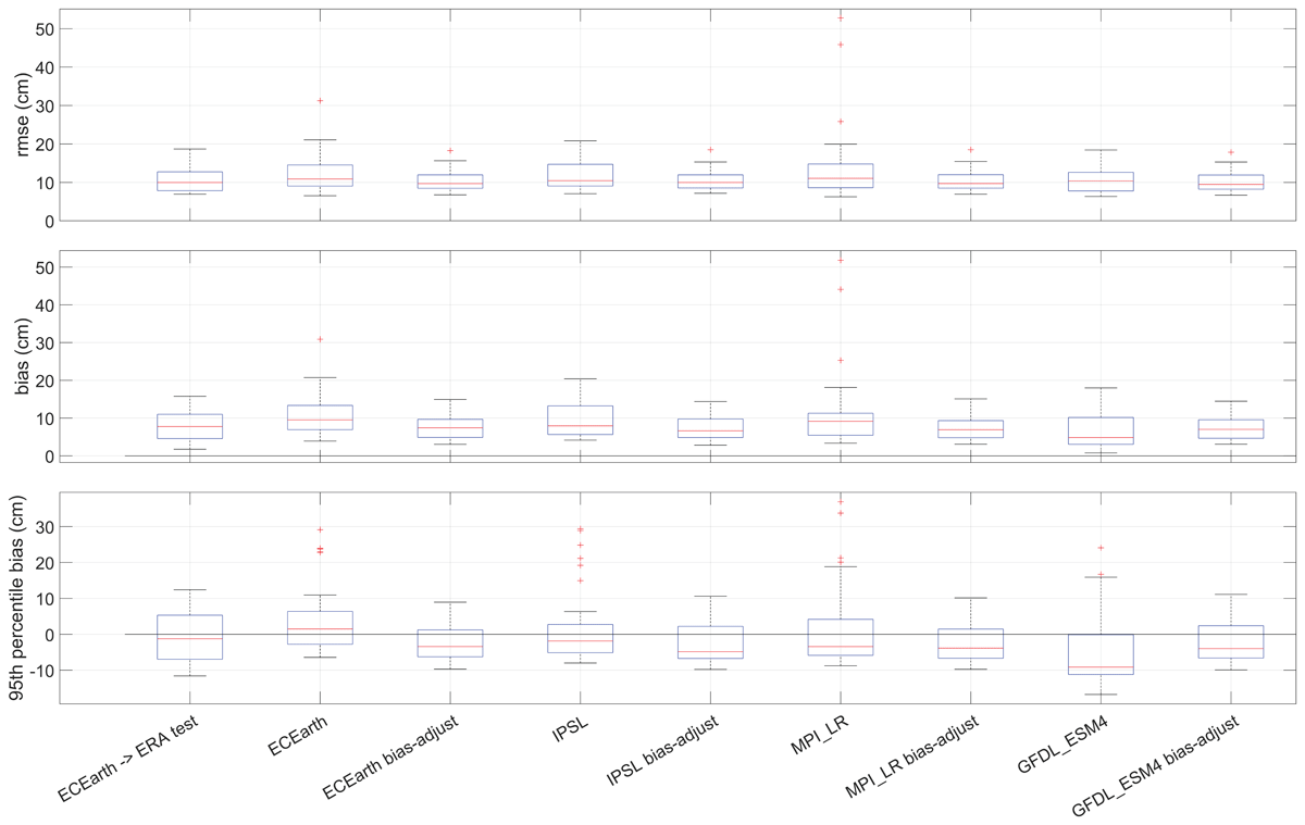
Figure 3
GOF metrics over the daily maxima time series of each RF model with three inputs (ERA, CMIP6, and CMIP6 bias adjusted) for the four climate models at each station. GOF metrics are calculated from the sorted scatter plots. ERA5 statistical coefficients are measured based on the testing period whereas CMIP6 and CMIP6 bias-adjusted statistical coefficients are based on the validation period (Table A1).
Across all stations, the GOF of the RF model for predictions based on ERA5 during the testing period (ERA test), as well as the four climate models with unadjusted and quantile-mapping bias adjusted inputs during the validation period, showed RMSE and bias values between 2 and 10 cm, and perc95-biases between 4 and 30 cm. Higher variability was observed for cmip_model predictions across the models compared to cmip_model bias-adjust predictions. ERA test predictions did not consistently provide the best GOF metrics based on the sorted scatter plots compared to cmip_model or cmip_model bias-adjust predictions. The accuracy of the CMIP6 unadjusted or CMIP6 bias adjusted datasets was therefore site-dependent and varied with the chosen climate model (Figure 3 and Figure A4). For instance, at the Finnish station “Pori Mäntyluoto Kallo”, the EC-Earth predictions showed the most accurate results, with a slight overestimation of the perc95-bias of 0.6 cm compared to an underestimation of –4.3 cm for the EC-Earth bias-adjust predictions. However, at this site, the GFDL-ESM4 bias-adjust predictions were more accurate than the GFDL-ESM4 predictions, with perc95-biases of –5.4 and –9.7 cm, respectively (Figure A4). Examining the scatter plots in more detail reveals that the prediction uncertainties generally align with the identity line, particularly for extreme highs compared to extreme lows (Figure A1 and Figure A2).
3.1.2 Storm tides RLs
Predicted storm tide RLs across the four climate models exhibited similar behavior and statistics for most stations. As previously noted, stations with short time series do not allow for optimal validation, resulting in high variability in GOF measures, with occasional divergence in the GEV distributions (highlighted with red circles in Figure A5). These stations are located in the south and east of the Baltic Sea, as well as the station Halmstad on the west coast of Sweden.
Overall, the RF method with random sampling (Dubois et al., 2024) allowed for improved RL estimation, showing RMSE values that are lower by around 25 to 35 cm on average, along with reductions in bias and perc95-bias by an average of 25 to 50 cm (Figure 4). RLs derived from the RF method with random sampling using ERA5 inputs showed the highest accuracy, with a median RMSE around 5 to 6 cm, a near-zero median bias, and a slightly positive median perc95-bias of 3 cm across the different stations (Figure 4). For each climate model, RLs based on the RF method with random sampling exhibited RMSE values typically within 35 cm and biases ranging from –35 to 25 cm. Depending on the chosen climate model and site, higher accuracy was achieved by applying the quantile-mapping bias adjustment as inputs to RFst(cmip_model) (Figure 4 and Figure A5). For example, EC-Earth predictions presented better GOF than EC-Earth bias-adjust, whereas GFDL_ESM4 bias-adjust were more accurate than GFDL_ESM4 for the station “Pori Mäntyluoto Kallo” (Table A1). In general, negative biases were observed, indicating a tendency to underestimate extremes (Figure A5). However, as shown in Figure A3 for the Finnish station “Pori Mäntyluoto Kallo” with the EC-Earth model, the uncertainties associated with the RF method with random sampling align with the identity line and fall within the 95th percentile confidence interval of the observations. This pattern is consistent across all sites and climate model.
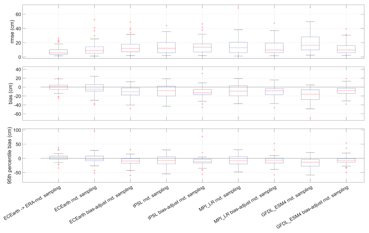
Figure 4
GOF metrics over the storm tide RLs of each RF model with three inputs (ERA, CMIP6, and CMIP6 bias adjusted) for the four climate models at each station where the GEV fit converges. GOF metrics are calculated from the sorted scatter plots for both the mean predictions and the RF method with random sampling (Dubois et al., 2024). ERA5 statistical coefficients are measured based on the testing period whereas CMIP6 and CMIP6 bias-adjusted statistical coefficients are based on the validation period (Table A1).
3.2 Atmospheric Characteristics of ESL
Atmospheric characteristics of ESL events were briefly evaluated based on sea level observations from each tide gauge independently. Within the Baltic Sea, ESLs have previously been described to reach up to 250 cm, with higher sea levels observed in the eastern and northern Baltic Sea regions and occasionally exceeding this threshold in the Gulf of Riga, located in the east of the Baltic Sea (Wolski et al., 2014). A similar spatial pattern, with higher 30-year RL values in the Gulf of Riga, Finland, the northern Baltic Sea, and around the Danish Straits, and lower values along the East coast of Sweden, was found by Lorenz and Gräwe (2023) based on a hindcast ensemble for the Baltic Sea. Pindsoo and Soomere (2020) reported that annual sea level maxima increased at rates ranging from 1.5 to 10 mm per year between 1961 and 2005 in the Baltic Sea with faster increases observed in the East and South-West regions.
Wind characteristics associated with ESL events, as defined in section 2.2.1, were outlined. Storm tides on the west coast of Sweden corresponded with westerly winds, while in the Bothnian Bay (northern Baltic Sea), they aligned with southerly winds. South-westerly winds drove storm tides along the west coast of the Baltic Sea, including the Gulf of Finland and Riga (Figure 5). Along the south and east coasts of Sweden, however, no single wind direction consistently correlated with ESL events, as these may arise from various directions (Figure 5). This may suggest that extremes at these stations are not driven to the same extent by local winds as at other locations. However, it could also be interpreted as a transition zone effect (along the south Swedish coast) or a sheltered zone effect (along the north-eastern Swedish coasts), as these areas are midway between the end-positions of north-easterly winds (impacting the southwestern Baltic coasts) and south-westerly winds (impacting the Bothnian Bay coasts), thereby being somewhat sheltered from those winds. Overall, winds associated with ESLs aligned with the prevailing winds at each station. Storm tide events exceeding the 99th percentile threshold were associated with stronger winds than those exceeding the 95th percentile threshold.
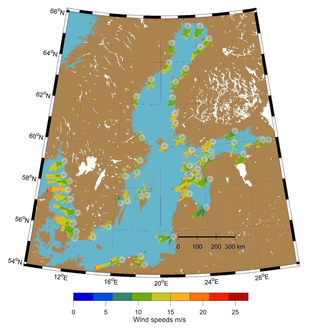
Figure 5
Characteristics of wind direction and wind speed (wind roses) from ERA5 reanalysis associated with ESL events defined as independent events with daily maxima sea level above the 95th percentile threshold value obtained from observation time series at each station over the co-occurring period (Table. A1).
The likelihood of observing ESL events that aligned with the prevailing wind direction was higher due both to the probability of such wind direction occurring and to the location of each site, where dominant winds are generally directed onshore, as storm surges arise from winds pushing water towards the shore. This analysis focused on wind characteristics observed on the same day as ESL events; however, other factors in this area also contribute to ESLs, including tides, which typically range from a few centimetres up to 40 cm during spring tides in the Skagerrak basin (Medvedev et al., 2013). “Preconditioning” of sea levels (Andrée et al., 2023; Weisse et al., 2021) is another phenomenon that influences ESLs in the Baltic Sea. Additional phenomena, such as meteotsunamis and seiches, also affect sea levels and may partially drive ESL events (Arneborg and Liljebladh, 2001; Hanson and Larson, 2008; Holthuijsen, 2007; Lorenz et al., 2024; Nesteckytė et al., 2024; Pellikka et al., 2020; SMHI, 2014; Wolski and Wiśniewski, 2023).
3.3 Historical (1850–2015) and projected Climate (2015–2100) of storm tides
To analyse changes in storm tides, the methodology outlined in section 2.2 was followed. Four climate models (EC-Earth, IPSL, MPI_LR, GFDL_ESM4) with historical and SSP2–4.5 climate scenarios were used to predict sea level daily maxima time series from 1850 to 2100. The results enabled the assessment of potential changes in storm tides, which may indicate increases or decreases in coastal flood hazard from storm tides at the local scale of each station, spatially covering most of the Baltic Sea. Figure 6 displays the difference in 50-year storm tide RL expected between the 2070–2099 and 1850–1879 periods, based on the ensemble mean of the four climate models. These storm tide RLs varied from a decrease of –6 cm to an increase of 8 cm, except the upper-Baltic Sea station of “Kemi Ajos”, which showed an increase of 17 cm (Figure 6, Figure 7, and Figure A6). Overall, changes in 50-year RL storm tides are expected at the sub-regional scale, with variations in local conditions. Out of the 59 stations, 25 showed minor changes ranging from –2 to +2 cm, primarily located within the Baltic Proper, the Bothnian Bay and the Gulf of Finland. Fifty stations showed changes from –5 to +5 cm, with half of those indicating an increase. Two stations exhibited a stronger decrease (Kolka, and Skanör), while seven stations demonstrated a notable increase. The west coast of Sweden in the Kattegat basin and the Bothnian Sea both displayed an increase in 50-year RL storm tides, which can potentially be linked to stronger westerly and southerly winds in those areas. Conversely, stations on the south coast of Sweden, the Gulf of Riga, and the mouth of the Gulf of Finland showed decreasing levels, which may be attributable to a general weakening of high wind speeds in these areas (Figure 6). Stations located close to one another with similar topographical characteristics (e.g. within channels, gulfs, or their mouths) generally experienced similar changes in storm tides, likely due to their exposure to the same meteorological phenomena at the synoptic scale that drive storm surges. Similar differences in 30-, 100-, and 200-year RLs were found across the different sites, yielding consistent conclusions. When comparing 50-year storm-tide RL differences between 2070–2099 and 1960–1989, a similar spatial pattern emerged, although with a stronger decrease for stations in the Bothnian Sea and south of the Bothnian Bay.
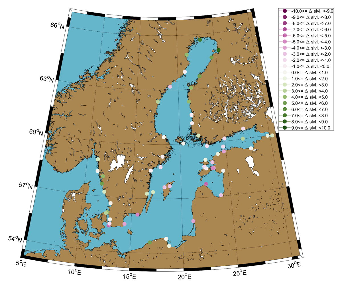
Figure 6
Difference values of the ensemble mean from the four climate models of the 50-year RL storm tide calculated between the 2070–2099 and 1850–1879 periods at each station (cf. section 2.2.3).
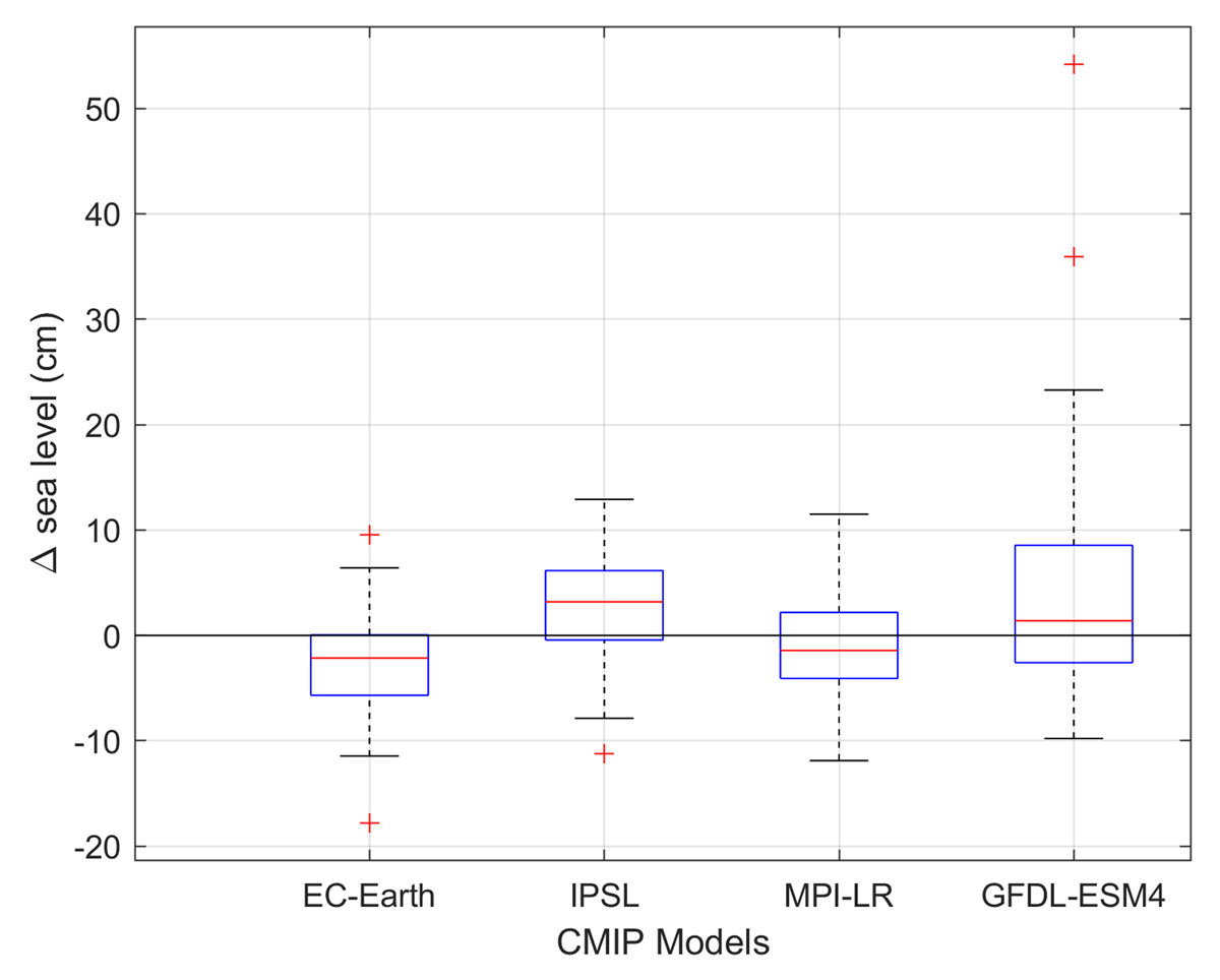
Figure 7
Box plots of the difference in 50-year RL storm tide between 2070–2099 and 1850–1879 at each station, grouped by climate model.
Figure 7 illustrates the variability in 50-year RLs, across all stations, between the four climate models between the 2070–2099 and 1850–1879. Each model exhibited considerable variability across stations, with differences typically within the range of 23–33 cm. Notably, the Finnish stations of “Oulu Toppila” and “Kemi Ajos” located in the uppermost part of the Bothnian Bay, showed higher variability up to 47 and 60 cm respectively, between EC-Earth (lowest value) and GFDL-ESM4 (highest value) (Figure A6 and Figure A7). This may be related to variations in the projected future wind speeds in the central parts of the Baltic Sea, where, as seen for the GFDL-ESM4 model, a change towards more southerly oriented extreme winds (>99th percentile) is seen (Figure A9a and Figure A9b). Eight stations exhibited less than 5 cm variability across models, including the Swedish station “Klagshamn” in the South of the Baltic Sea, which presented the smallest inter-model spread of only 2.3 cm. Overall, EC-Earth results showed a stronger decrease in storm tide RLs in the future, with differences ranging from –18 to 10 cm and a median value of –2 cm across sites (Figure 7 and Figure A6). The GFDL-ESM4 model generally indicated an increase in storm tide RLs, with a positive median of 1 cm and high variability ranging from –10 and 54 cm across stations. The IPSL and MPI-LR models showed less variability in the storm tide RL changes, with values spanning from –11 to 13 cm and –12 to 12 cm, centred on median values of 3 and –1 cm, respectively (Figure 7 and Figure A6). This variability may be attributable to EC-Earth projecting fewer storms or a general weakening of strong wind speeds in the future, whereas GFDL-ESM4 projects stronger winds in the future (Figure 8). IPSL and MPI-LR did not indicate important future wind speed changes in these regions. Another factor could be shifts in prevailing wind directions associated with high wind speeds, which could alter storm surges at specific locations and potentially relate to large-scale atmospheric circulation changes, associated with a possible northward shift of storm tracks over the North Atlantic (Meier et al., 2022b; Rutgersson et al., 2022). Natural variability appears to dominate over warming trends driven by anthropogenic emissions at most stations, as indicated by the larger standard deviations compared with the linear trends observed across the stations (Figure A8). Exceptions include the “Kemi-Ajos” site for GFDL-ESM4 and EC-Earth, where stronger trends were evident. Specifically, the stations “Kemi Ajos” and “Oulu Toppila” showed absolute linear trends in the 50-year storm tide return level (RL) from 1850 to 2100 exceeding 1 mm/year, with trends of 2.4 mm/year and 1.7 mm/year for GFDL-ESM4, and –1.8 mm/year and –1.5 mm/year for EC-Earth, respectively. Studies by Hieronymus and Kalén, (2020) and Dangendorf et al., (2016) have demonstrated the substantial influence of natural variability on RL estimates, with significant differences arising from the inclusion or exclusion of specific years in both short (about 20 years) and longer time series. These findings highlight the high natural variability in storminess within the region. Considering this natural variability and inter-model differences, the observed trends in this area are likely to be predominantly driven by natural variability rather than anthropogenic warming.
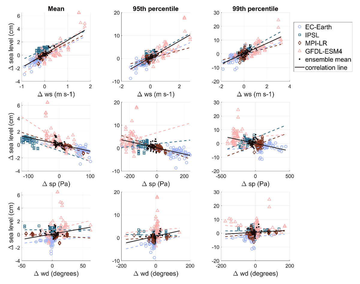
Figure 8
Scatter plots of the difference values of the mean, 95th and 99th percentiles (for each column) from the atmospheric variables: wind speed (ws), wind direction (wd), and the 5th and 1st percentiles of surface pressure (sp) (x-axes) against sea level (y-axes), calculated between 2070–2099 and 1850–1879 at each station, and for each climate model, as well as for the ensemble mean.
3.4 Link between atmospheric drivers and storm tide changes
This section aims to provide a better understanding of the causes leading to storm tide changes by analysing changes in atmospheric drivers. The focus is on changes between the periods 2070–2099 and 1850–1879. Figure 8 presents the differences in the mean, 95th, and 99th percentile values calculated over these two 30-year periods for the optimal sea level prediction at each site independently, and for the wind speed and corresponding wind direction, as well as the differences in the mean, 5th, and 1st percentile values for the surface pressure. Each climate model is analysed individually, as well as the ensemble mean.
From the plots, a significant correlation can be seen between wind speed and storm tide changes, with higher wind speed differences associated with higher sea level differences. Spearman correlation coefficients range from 76% (99th percentile) to 81% (95th percentile), indicating a decrease in the linear correlation for the most extreme events (i.e. above the 99th percentile), likely due to non-linear effects (Figure 8). Overall, with linear fitting, an increase in wind speed of 1 m s–1 drives an increase in sea level of around 2.1, 3.6 and 3.8 cm for the mean, 95th, and 99th percentile difference values, respectively. Thus, for a similar change in wind speed, higher sea level differences are expected in extreme events. Surface pressure shows a weaker linear correlation with sea level, though still significant, with Spearman coefficients between 49% and 63% for the 99th and 95th percentiles, respectively. A decrease in surface pressure drives an increase in sea level, likely due to the inverted barometric pressure effect, usually referring to a change of 1 cm per hPa, consistent with linear fittings applied to our datasets across the models (Figure 8). Low correlation coefficients ranging from 9% to 23% for the 99th percentile and mean values, respectively, were found in the relationship between wind direction and sea level, indicating that changes in wind direction do not systematically drive sea level changes. Wind speed therefore emerges as the main driver of changes in storm tides, with surface pressure acting as a secondary driver, as also found by Lorenz et al. (2024), while wind direction appears to play a minor and more localized role in influencing sea level changes in this region. However, this is based on a single-variable approach, whereas in a multivariate analysis, the interplay between variables such as wind speed and direction becomes relevant. Lorenz et al. (2024) also find that Atlantic sea levels significantly affect storm surges in the Skagerrak and Kattegat basins.
Interestingly, different patterns emerge when looking at each model separately, where GFDL-ESM4 shows a higher variability for all variables. As highlighted in section 3.3., EC-Earth presents the strongest decrease in sea level between the two periods (2070–2099 and 1850–1879) across all values (mean, 95th, and 99th percentiles). This decrease can be linked to reductions in both daily mean wind magnitudes and extreme wind speed values at most stations, as well as an increase in surface pressure (possibly due to more anticyclonic conditions). GFDL-ESM4, by contrast, shows a stronger increase in wind speed and a decrease in surface pressure during extreme events at most sites compared with the other models. When looking at the mean values differences over the time periods, IPSL exhibits a more substantial decrease in surface pressure of around 100 Pa, resulting in a slight increase in sea level. This trend is similarly reflected for the extremes when looking at the surface pressure. However, IPSL and MPI-LR do not show the same magnitude of changes in wind speed as GFDL-ESM4 and EC-Earth, resulting in relatively minor changes in storm tides for IPSL and MPI-LR. MPI-LR presents a slight overall increase in surface pressure, which can be linked with a slight decrease in sea level; however, as noted in section 3.3., this outcome is site-dependent. Wind direction may change significantly between models (Figure 8), especially in GFDL-ESM4 and EC-Earth, when examining extreme values for stations located in the Bothnian Bay and Bothnian Sea (north of the Baltic Sea) as displayed in Figures A9a and A9b, showing the change in wind roses at each station for wind speed events above the 99th percentile between 1850–1879 and 2070–2099 for GFDL-ESM4. This variation might relate to projected reductions with high confidence in sea ice conditions (Meier et al., 2022b) by the end of the century, as sea ice acts as a shield to the sea surface from wind forcing, thereby impeding the development of ESLs, and has been found to impact storm surges in the North of the Baltic Sea (Lorenz at al., 2024). At other sites, wind direction changes range from –10 to 25 degrees, –30 to 20 degrees, and –60 to 60 degrees for the mean, 95th, and 99th percentiles, respectively.
The dashed correlation lines highlight notable differences in how each model captures the relationships between atmospheric drivers and storm tide changes (Figure 8). The strong correlation observed across models (solid line) is partly due to the inclusion of multiple models, leading to a broader span of outcomes, which may exaggerate the overall correlation. When only one model is included (each dashed line), the correlation decreases and the range of values becomes smaller. This variability underscores the importance of inter-model differences in predicting storm tide changes. Including even more models could offer further insights, although this must be balanced against processing time and available resources.
3.5 Future projections of high sea level at three sites
When considering local relative mean sea level changes due to sea level rise and glacial isostatic adjustment (Weisse et al., 2021), a more realistic picture of ESL changes in the future can be obtained. For example, under SSP2–4.5, the stations “Kalix”, “Stockholm”, and “Göteborg” project changes to the relative mean sea level (blue bars in Figure 9) by approximately –19, +8, and +27 cm by 2080, respectively, compared with the reference period of 1995–2014 (SMHI, 2020). When adding projected changes in storm tides based on the 50-year RL difference between the 2060–2094 (centred around 2080) and 1985–2014 periods (red bars in Figure 9) for the ensemble mean, a lower total ESL is expected by 2080 of –21 cm for Kalix, no notable change in the 50-year RL storm tide for Stockholm, leading to a total increase of 8 cm, and an increase of up to 30 cm for Göteborg (Figure 8). Larger uncertainties are observed for storm tides projections compared to estimates of the local relative sea level rise. However, when aggregating the 95th percentile upper band of those uncertainties, a potential increase in ESL difference of around 27 cm for Kalix, 53 cm for Stockholm, and 70 cm for Göteborg is possible (Figure 9), based on the climate model ensemble mean. Despite some variability across the climate models, future changes in storm tides may alter ESL projections in the Baltic Sea. For example, based on the ensemble mean storm tide level projections, 12%, 2%, and 10% of projected changes by 2080 are due to storm tide changes at Kalix, Stockholm, and Göteborg stations, respectively (Figure 9).
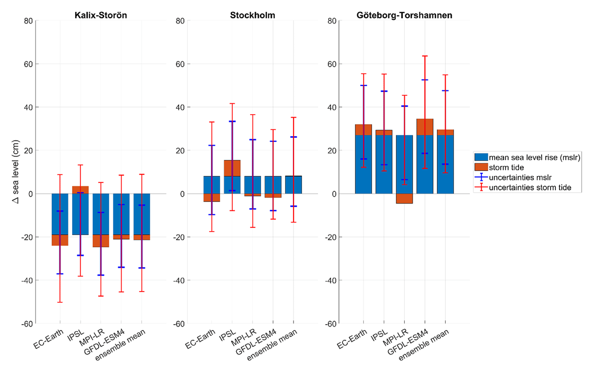
Figure 9
Difference values of the 50-year RL storm tide calculated between the 2065–2094 and 1985–2014 periods displayed with projected local mean sea level changes by 2080 under SSP2–4.5 (SMHI, 2020) at stations Kalix, Stockholm, and Göteborg. Uncertainties associated with each projection are shown as error bars (95th percentile confidence interval) centred on the cumulative total sea level.
4. Limitations
This work is based on datasets of observational time-series, which may sometimes have a relatively short length (Table A1), potentially resulting in high uncertainties from the RF model due to the difficulty for such models to predict sea levels outside the range seen in the training data (Dubois et al., 2024; Hengl et al., 2018; Tyralis et al., 2019). This limitation also introduces uncertainties for those same stations during the testing and validation phase, which may be too short to contain proper comparison grounds for extreme events. However, stations with longer observation time series, once validated, enhance confidence in the methodology. Confidence in stations with shorter time series increases when nearby stations with longer time series yield similar results, as observed in our analysis. The use of GEV fit only can also be a limitation but Lorenz and Gräwe (2023) found that both the GEV and the Generalized Pareto Distribution reproduce similar extreme value distributions at different tide gauges around the Baltic Sea based in hindcast assessments. The decision not to de-tide the time series, particularly in the Kattegat/Skagerrak region where tides can reach up to 40 cm during spring tides, may introduce biases in the RF model’s performance. However, given the relatively low tidal range across most of the Baltic Sea, this approach was chosen to maintain consistency across stations and to avoid introducing additional pre-processing steps. Although oceanographic and atmospheric timescales differ, the inclusion of time-lagged wind and pressure variables in the RF model was briefly tested. However, initial results did not indicate significant improvements in predictive performance. This could be due to the relatively short memory of atmospheric forcing in storm tide generation within the Baltic Sea. Nonetheless, future studies could further investigate the optimal selection of time-lagged inputs, particularly in regions where meteorological influences persist for longer durations. While atmospheric predictors such as wind speed, wind direction, and surface pressure were selected for simplicity and data availability, the absence of sea ice coverage as a predictor represents a limitation, particularly in the northern Baltic. Sea ice modulates storm tides, and its long-term reduction due to climate change could influence future predictions. Although wind conditions partially account for the effects of sea ice, this aspect warrants further investigation. The RF model was validated directly against observations rather than compared to state-of-the-art ocean models. While this ensures validation with the least biased dataset available, a comparison with numerical ocean models during the ERA5 period could provide additional insights into the model’s predictive skill, particularly for extreme events. Future work could assess the RF model’s performance relative to traditional hydrodynamic models, particularly in terms of RMSE and bias in extreme value predictions. Also, the quantile-mapping bias adjustment method may affect trends and therefore have a large effect on climate driven trends (Cannon et al., 2015). Here, we found a high significant correlation between linear trends with and without quantile-mapping bias adjustment method across models and stations, and with near-zero trends (<1 mm/year), this effect can be considered negligible. Nevertheless, alternative bias correction approaches exist, such as empirical quantile mapping (Byun and Hamlet, 2024) or trend-preserving bias correction (Hempel et al., 2013), and their applicability to this study could be explored further in future research. The high internal variability in the Baltic Sea at multidecadal scales prevents a straightforward detection of changes in ESL (Lang and Mikolajewicz, 2019). Likewise, the high inter-model variability of the results underscores the uncertainties related to future storm tide projections.
The choice of climate scenario is another limitation and source of uncertainty (Hieronymus, 2020). SSP2–4.5 represents a mid-range scenario, estimating a global warming of 2.7°C by 2100 with emissions peaking around mid-century. Although the Intergovernmental Panel on Climate Change (IPCC) does not assess the likelihood or feasibility of specific carbon dioxide emission scenarios, such information is often essential for policymakers and end-users (Ho et al., 2019). Hausfather and Peters (2020) argue that current energy sector trends and policies align with the SSP2–4.5 scenario. Likewise, Den Elzen et al. (2022) indicate that climate change mitigation efforts would need to be significantly intensified to achieve a low-emission pathway, suggesting that SSP2–4.5 remains the most probable emission scenario under existing policies. The methodology presented in this study can be generalized to global scales and applied at other sites to retrieve local estimates of storm tides, while its performance might vary with variations in local oceanographic and meteorological conditions.
5. Summary and conclusions
This study assesses predictions of storm tides within the Baltic Sea from the historical period of 1850 to 2015 to the future period of 2015 to 2100 under the climate scenario SSP2–4.5, mainly focusing on the comparison between pre-industrial times 1850–1879 and 2070–2099. Based on our analysis, we conclude that:
Overall, no major changes in storm tide RLs are expected, as the ensemble mean values appear to remain within the range of natural variability. Stations located at the west coast of Sweden and in the Bothnian Sea show an increase in storm tide RLs between the 1850–1879 and 2070–2099 periods up to 10 cm (although +20 cm for “Kemi Ajos” station), while station at the south coast of Sweden, the Gulf of Riga, and the outer Gulf of Finland, show a slight decrease down to –6 cm.
High inter-model variability in the atmospheric variables of climate models results in large uncertainties in storm tide projections.
Stations located close to each other experience similar changes in storm tide trends, which highlights a regionalization effect likely associated with comparable synoptic scale meteorological phenomena.
Projected storm tide changes may alter projected local ESL changes by up to 12% across the three stations in this analysis, based on the 50-year storm tide RL, although storm tide projections hold a greater uncertainty.
Future projections of ESL, with regard to both magnitude and uncertainty, is essential in the preparation towards future coastal flood hazards. This study provides insights into potential storm tide changes by the end of the century at different stations in the Baltic Sea and underscores the importance of considering storm tide changes alongside local mean sea level changes to predict coastal flood levels in the future.
Additional File
The additional file for this article can be found as follows:
Acknowledgements
The work forms part of the project: Extreme events in the coastal zone – a multidisciplinary approach for better preparedness.
Competing Interests
The authors have no competing interests to declare.
Author Contributions
KD conducted the analysis. KD prepared the manuscript with contributions from all co-authors.