
1. Introduction
Ocean fronts are important phenomena in the world oceans and coastal regions (Mauzole, 2022). They are characterized by strong sloping interfaces from the surface to depth, with strong temperature, salinity, and density gradients including vertical and horizontal shears where upwelling and downwelling take place along the frontal interface, which is important for vertical transport of heat, salt, and biological properties (Zhu et al., 2024). The frontal boundary is caused by convergence of different water masses. It is meandering where eddies are generated due to baroclinic instabilities including the generation of internal waves important for turbulence and mixing in the ocean, see, for example, reviews by Johannessen (1975), Alford et al. (2016), Mahadevan (2016), McWilliams (2019), and Taylor and Thompson (2023).
The Maltese Ocean Front in the Mediterranean Sea has been the subject of observational and modelling studies for decades, with the most intensive observational campaigns during the early 1970s. This paper revisits a unique high-resolution legacy dataset from an integrated experiment of the Maltese Ocean Front (MAYFROST) on the shelf-slope east of Malta in May–June 1971. The goal at that time was to study the location, structure, and dynamics of this ocean front. The MAYFROST Experiment is described by Johannessen et al. (1971) in a preliminary technical memorandum. The first part was carried out by aerial remote sensing observing the sea-surface temperature (SST) by Airborne infrared-red thermometry (ART) including dropping Airborne Expendable Bathythermographs (AXBTs) from the plane and in-situ observations from a ship (Briscoe et al., 1974). Prior to the ship mapping of the front, ART flights were made on 10 and 11 May, where the result was communicated to the ship team, before the large-scale mapping started on 13 May, and completed on 22 May. The second part of MAYFROST was at that time a novel approach where high-resolution oceanographic sections of temperature, salinity, and density structure were repeated seven times across the front in the same location along 36°N latitude from the ship with a salinity/temperature/depth probe (STD) and Expendable Bathythermographs (XBTs) with station spacing of 1–2 km during a 10-day period, 23 May to 1 June. Current measurements and internal wave observations were obtained from anchored buoys in the sloping interface of the front preliminarily reported in a memorandum by Johannessen (1976).
In Johannessen et al. (1971), Briscoe et al. (1974), and Johannessen (1976), these observations showed that the Maltese Front was located from the southern part of Sicily, along the 15°20’ E longitude, caused by the intrusion of the Atlantic Water between Sicily and Malta, converging with the Ionian Sea Water, thereafter curving southeastward at 35°20’ N, well correlated and controlled by the shelf-slope east of Malta. The front meandered, and upwelling and downwelling took place along the frontal interface. Furthermore, the frontal interface was broken up due to a strong wind event in the later part of the experiment. However, so far only the surface temperature by ART and surface temperature measurements from the ship have been published (Briscoe et al., 1974).
Other limited investigations of this front during summer were first reported by Woods and Watson (1970) and summarized in Woods (1972), where ART SST was used to locate the front where three XBTs sections were done from a fast-moving boat. Based on these few sections, they interpreted that upwelling and downwelling took place. Woods, inspired by a paper by Hoskins (1971) dealing with atmospheric frontogenesis, suggested a conceptual model where equal upwelling and downwelling took place at the node of the frontal wave, and that upwelling occurred at wave crest and downwelling at the wave trough. Furthermore, a modeling study of the Maltese Front was done by Adamec and Garwood (1985), inspired by the observations from the MAYFROST Experiment (Johannessen, 1976). They focused their modeling study on the front’s response to the strong wind event in the later part of the MAYFROST Experiment. They also showed that inertial waves could be generated by the front, which was recently confirmed by Chunchuzov et al. (2023) by using the internal wave observations from the two thermistor chain buoys anchored in the frontal interface during the MAYFROST Experiment (Johannessen, 1976).
A more recent investigation in the Sicily–Malta region was done by Nardelli et al. (2001) during the SYMPLEX Experiment in 1998 in the northern region of the MAYFROST Experiment, although they did not use the term Maltese Ocean Front. They called the front the Atlantic–Ionian Sea stream. From one large-scale non-synoptic mapping, they showed a similar surface salinity pattern (their Figure 4) as already reported by a non-synoptic surface salinity mapping of the Maltese Front by Briscoe et al. (1974, their Figure 6). (The term ‘synoptic’ in oceanography is according to the Encyclopedia-Free Dictionary: ‘The study of physical parameters of the ocean through the analyses of simultaneous observations from many stations’). Their main experiment was a detailed three-day mapping of the ocean structure with 45 stations using a salinity/temperature/depth probe (CTD), including current from a ship-mounted Acoustic Doppler Current Profiler (ADCP), along west–east section in a box between 36.25° and 36.85° N and 15.4° and 16.0° E with 8 km resolution. Their box was just north of MAYFROST repeated seven detailed sections across the front in 1971 (Johannessen, 1976). Their west–east sections of temperature–salinity–density in the box showed only the medium scale structure of the frontal interface, but not the detailed structure as shown by Johannessen (1976), where the STD and XBT stations spacing were down to 1 km across the frontal interface, compared to the 8 km station spacing by Nardelli et al. (2001). Furthermore, they used three days to observe the box which makes it difficult to interpret the 3-D synoptic ocean structure, due to the temporal variability in this region. They focused their study on meanders and eddies in this Atlantic–Ionian Sea stream where they show that vertical velocity in an area of upwelling was in the order of 15 m/day in the meander ridge (crest) and downwelling of 17 m/day in the meander trough, in close agreement with Wang and Ikeda (1997) general numerical simulation study.
Another investigation in this frontal region was done by Drago et al. (2010, their Figure 8) where they show an IR satellite image of surface temperature covering the Strait of Sicily, the Malta region and the Ionian Sea on 22 July 2002. This image also showed that the Maltese Ocean Front meanders and spins off eddies, well correlated with the shelf-slope east of Malta. Furthermore, it showed that the intrusion of the Atlantic cold water broke up the front southeast of Malta, very similar to the ART observations by Briscoe et al. (1974). However, they were not studying the Maltese Front, but at least they used the name of it when they showed the IR image. Previous to this, Drago et al. (2003) implemented a 3-D model for the Malta shelf area studying the ocean circulation, but again no detailed study of the Maltese Ocean Front. Pinardi et al. (2015) in a modeling study and Suarez et al. (2019) in a comprehensive remote-sensing study of the surface circulation in the Malta–Sicily region, showed that the Atlantic inflow of the water south of Sicily turns southwards along the Malta shelf-slope before turning southeastward into the Ionian Sea south of Malta, both during summer and winter, again similar to the ART and surface salinity observations by Briscoe et al. (1974) during summer season. However, again no detailed study of the Maltese Ocean Front was done. All of the above-mentioned papers related to the Maltese Ocean Front region, spanning from 1970 to 2019, show that the Maltese front is located along the shelf-slope east of Malta, indicating that this is a permanent frontal zone. Finally, Poulain et al. (2023) and Oddo et al. (2023) studied internal wave tidal dynamics on the Malta shelf, with no special study of the Maltese Ocean Front.
The memorandums by Johannessen et al. (1971) and Johannessen (1976) have not been published in a journal, only the surface temperature by ART and towed ship temperature observations by Briscoe et al. (1974), a modelling study by Adamec and Gatwood (1985) and a recent analysis of the internal wave observations from the MAYFROST Experiment (Chunchuzov et al., 2023). Since MAYFROST in 1971, the only detailed study of the northern part of the Maltese Ocean Front was done by Nardelli et al. (2001) during the SYMPLEX Experiment in 1998, but at a coarser scale than the MAYFROST Experiment. Therefore, the integrated case study of the Maltese Ocean Front during the MAYFROST Experiment in 1971 is still the most detailed one of this front describing upwelling and downwelling and a rare case study of an ocean front response to a strong downwind event from the northwest along the front.
The present paper deals therefore with a complete descriptive study of the MAYFROST Experiment. Section 2 describes the ocean frontal location, section 3 the frontal structure, upwelling and downwelling including the response to a strong wind event, section 4 the frontal dynamics, section 5 the discussion, and 6 the summary and conclusions.
2. Ocean Frontal Location
The Maltese Ocean Front study region and the underlying bathymetry is outlined in Figure 1. The first large-scale mapping of the sea-surface temperature (SST) east of Malta and the Ionian Sea was done on 10 May 1971 (Figure 2) by airborne infra-red thermometry (ART) by an US Navy P3 Orion plane during a 8-hour flight, of which a few hours were used for a quasi-synoptic location of the front north of 35°30’ N latitude up to the southern tip of Sicily and between 15° and 16° E longitude, under very calm wind conditions (Briscoe et al., 1974). The ART-SST location of the front, which had an SST change of more than 1°C over a few kilometers (km) with a meandering structure, was established from Sicily down to approximately latitude 34°20’ N. But here it was broken-up between latitudes 35°10’ and 35°30’ N and 15°30’ E longitude caused by the intrusion of slightly colder Atlantic water of less 16.6°C compared with the SST of the Ionian Sea water east of the front of more than 17.5°C in the beginning of the MAYFROST Experiment. Note also the indication of an eddy in the norther part at 36°30’ N with a temperature of less than 16°C in the center with a scale of about 20 km.
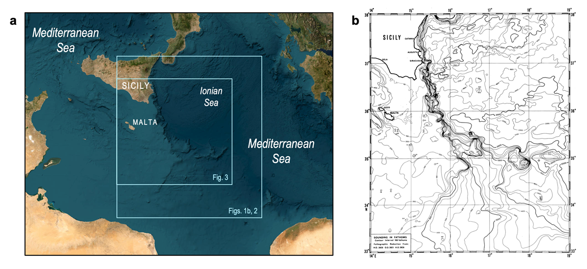
Figure 1
a, Map of the study area, with frames indicating the boundaries of the maps in Figures 1b, 2 and 3. Source: National Centers for Environmental Information (NCEI), Bathymetric Data View, World View, ESRI base map. b, Bathymetry of the region east of Malta with contour interval in 100 fathoms. Source H.O. 3920, O.O. 3921, H.O. 3926.
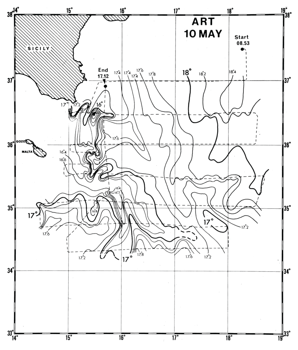
Figure 2
Large- scale mapping of the sea-surface temperature (SST) east of Malta and in the Ionian Sea on 10 May 1971 by Airborne infra-red thermometry (ART) by a US Navy P3 Orion plane during an 8-hour flight of which 5 hours were used for a quasi-synoptic location of the Maltese Ocean Front up to the southern tip of Sicily between 15–16° E longitude. [Source: Briscoe et al. (1974), Figure 1].
The salinity of the colder Atlantic water was less than 37.30 psu compared to the warmer Ionian Sea water with more than 38.0 psu east of the front (Figure 3), mapped by the SACLANTCEN Research Vessel MARIA PAOLINA G using towed thermistors at surface and five m, expendable temperature probes (XBTs) and 2000 surface water samples every 2.3 km for salinity determination during the period 13–22 May, based on guidance from the SST ART mapping on 10 May (Figure 2). During this mapping period the wind conditions continued to be very calm, but due to diurnal heating measured from the ship being up to 2°C in the immediate surface layer (Briscoe et al., 1974), the surface salinity map (Figure 3) is more conservative than the SST over this 10-day period. However, this mapping was not synoptic. Nevertheless, the salinity map also clearly shows the intrusion of the Atlantic water between Sicily and Malta, converging with the Ionian Sea water, steered by the shelf-slope topography (Figure 1b), which is located in a north-south direction between Sicily and north of 35°30’ N bending into the deeper channel in a southeast direction into the Ionian Sea. It is the intrusion of the Atlantic Water between Sicily and Malta converging with the Ionian Water, steered by the bathymetry which create this frontal zone, consistent with the southward current of 40–50 cm/s observed in the surface Atlantic layer from the anchored current meter array at 36° N latitude and 15°22’ E longitude (Figure 6a, Table 1). This is also similar to the inflow of Atlantic Water modeled by Pinardi et al. (2015) and observed by Suarez et al. (2019). An eddy is indicated with high salinity of more than 38 psu between 35°05’–35°25’ N latitude and 15°30’–15°55’ E longitude with the heavier Ionian Sea water in the center (Figure 3), indicating a cyclonic circulation with a scale of about 35 km. This eddy is spun off from the instability of the meandering front, normal in frontal regions; see reviews by, e.g., McWilliams (2019) and Taylor and Thomsen (2023).
Table 1
Velocities versus depth 5–15–30–60 m. Daily averages: Start at 15 hours on 27 May completed at 12 hours on 30 May 1971.
| DEPTH | DAY 1 | DAY 2 | DAY 3 | |||
|---|---|---|---|---|---|---|
| V CM/S | DIR.* | V CM/S | DIR. | V CM/S | DIR. | |
| 5 | 45 | 187 | 41 | 203 | 53 | 189 |
| 15 | 39 | 197 | 38 | 211 | 46 | 202 |
| 30 | 31 | 195 | 31 | 205 | 33 | 201 |
| 60 | 7 | 169 | 8 | 182 | 7 | 171 |
[i] * dir. = direction towards in degrees [Modified from Johannessen (1976), Table 1].
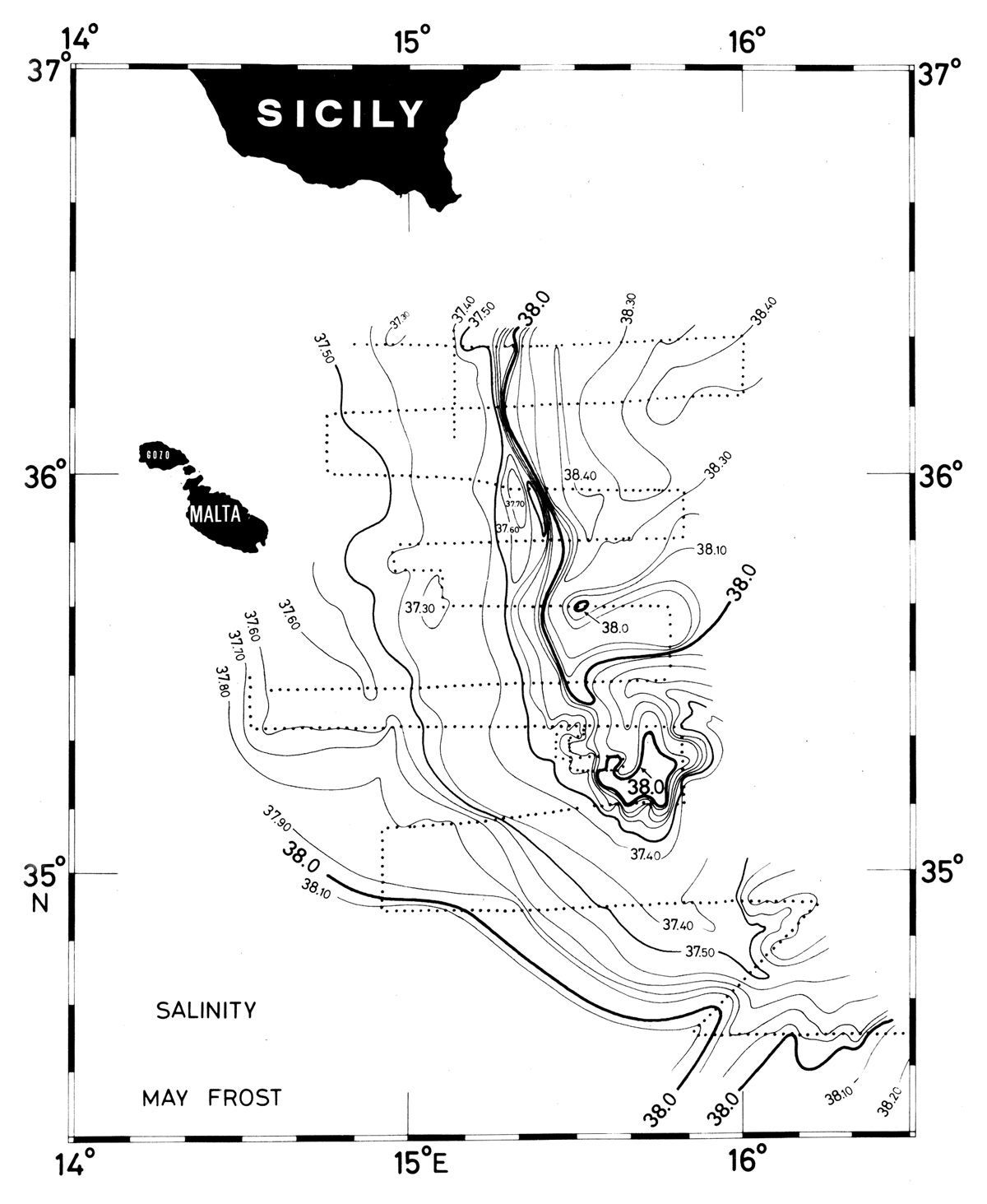
Figure 3
Surface salinity map of the frontal region east of Malta during the period 13 to 20 May 1971. The surface salinity was sampled by the ‘bucket method’, n = 2000, and the salinity was determined onboard the research vessel with a laboratory salinometer. The dots indicate the observations with a sampling rate for each 2.3 km, during a very calm period. [Source: Johannessen (1976), Figure 1].
3. Frontal Structure, upwelling and downwelling
Based on mapping of the front, the next part of the investigation dealt with observations of the front’s oceanographic structure by perpendicular sections of temperature, salinity and density (using STD and XBT probes) across the front by the ship during the period from 23 May to 1 June including anchoring a current-meter array and three thermistor chains during the period 27–30 May 1971. The frontal location was observed before the ship investigation by a detailed nearly synoptic mapping of the SST by the ART equipped airplane on May 19 during a period of 6 hours, with less influence of the diurnal heating of the surface. During this period the wind condition continued to be very calm up to late on 27 May when the wind suddenly increased nearly as a step function with peak values of 14–21 m/s from northwest, nearly along the front with the heavier water on the left side of the down-front wind forcing, averaging to 6–11 m/s for the remaining period of the experiment (Johannessen et al., 1971, p. 6).
The ART SST on 19 of May (Figure 4) was observed with 19 sections, 9 km apart during a period of 6 hours, which gave a detailed mesoscale nearly synoptic mapping of the front. The frontal boundary meandered with wavelengths varying between 15–30 km and a wave width of about 20 km. The meandering front was well correlated with the shelf-slope which has the same width as the frontal width from the edge of the shelf to the deep ocean (Figure 1b), including a similar waviness of the bottom topography as the front. The temperature changed by about 1°C over a distance of 2–4 km across the frontal boundary. The two patches of colder water of less than 17°C on the western crests of the frontal boundary, in the central part (35°40’ N) and southern part (35°10’ N) indicated that upwelling took place, as generally modeled by Wang and Ikeda (1997), also clearly shown later in the ocean vertical structure (Figure 6). The cold circular patch of less than 17.2°C in the center in the northern part west of the front, indicated an eddy with a scale of 20 km with anticyclonic rotation as also indicated in ART SST on 10 May (Figure 2). Comparing features of the frontal meander between the ART SST between 10 and 19 May (Figures 2 and 4) indicates the frontal wave propagation. A trough at 36°28’ N on May 10 had moved to 36°15’ N on 19 May, giving a southward propagation of 13 min. latitude, and another trough at 35° 40’ N which moved to 35°30’ N, giving a 10 min. latitude southward propagation and finally a crest at 35°50’ N which moved to 35°43’ N, giving a 7 min. latitude southward propagation. This gives an average southward propagation of the frontal wave of 10 min. latitude over 9 days, of about 2.1 km/day, equal to 2.4 cm/s. This is about 5% of the surface flow as observed from the anchor current meter array (Table 1) in the same order as the model result from Wang and Ikeda (1997).
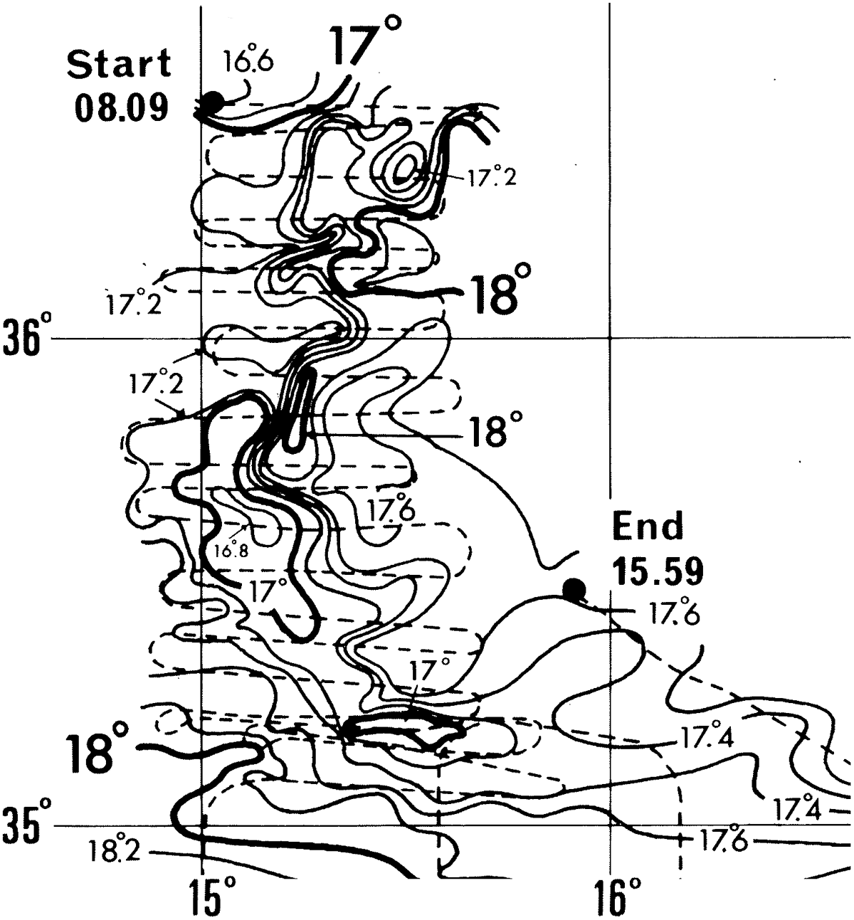
Figure 4
Detailed quasi-synoptic sea-surface temperature as obtained by an Airborne infra-red thermometry (ART) equipped airplane on 19 May 1971 during a period of 6 hours. Note the cold patches of less than 17°C in the middle of the figure and in the southern part which indicate upwelling along two crests of the meandering front during very calm wind conditions and the eddy structure with temperature of less that 17.2°C in the northern part of the figure, spun off from the front. [Source: Johannessen (1976), Figure 2].
It should also be mentioned that several of the ART-SST traces on the original strip chart recorder on the P3 ART plane across the front were extremely sharp, which in several of the cross sections showed a transition from one water mass to the other in less than 50 m (Briscoe et al., 1974, Figure 8c, p. 256), indicating that the temperature gradient is much stronger than shown in the interpolated ART SST map (Figure 4).
Based on the ART SST map (Figure 4) a time series of 7 sections of the ocean structure perpendicular to the front along latitudes between 35°58’ and 36° N were started on 23 May with the objective to study how the meandering frontal structure varied in time along this section. The temperature, salinity and density were observed by 3 STD and 4 XBT sections (Figure 5), with very dense station spacing in the frontal interface region, in the order of about 1 km or less. (Station spacing is marked with bars on the top of the figures, and longitude and time on the bottom of the figures). The current meter array was anchored later, west of the surface interface of the front (marked on Figure 6a) on 27 May and recovered on 30 May, sampling current at 5–15–30–60 m.
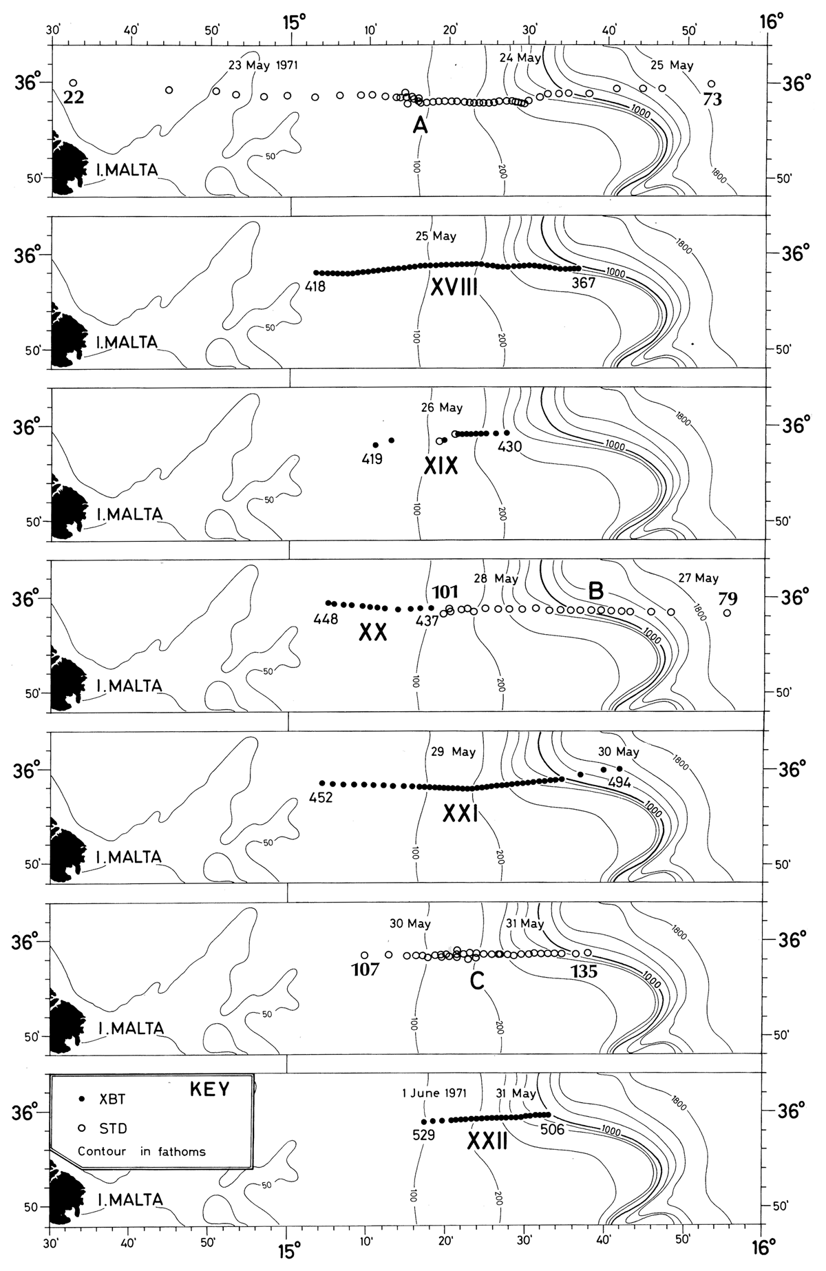
Figure 5
Programme of observations of the ocean structure of the Maltese Ocean Front during the period 23 May and 1 June 1971 by use of a a Bisset and Bergman 9060 temperature, salinity and density probe (STD) interfaced with a shipborne computer, giving values of temperature, salinity and density every 0.5 m in the upper 100 m and 1.5 m below 100 m. Expendable temperature probes (XBTs) were used to observe the temperature structure in a quasi-synoptic mode dropped from the moving ship. [Source: Johannessen (1976), Figure 3].
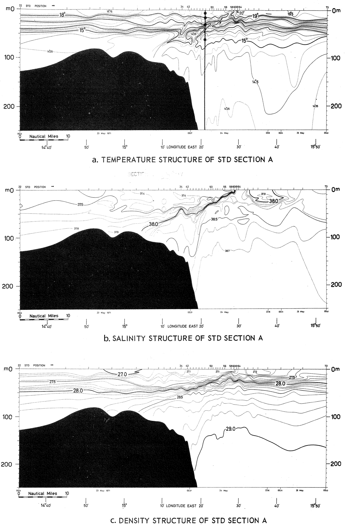
Figure 6
a, Temperature, b, salinity and c, density (STD) Section A on 23 to 25 May 1971; for position see Figure 5. The current meter array is marked on Figure 6a, but it was anchored only during a 3-day period 27–30 May. Dots mark the depth at 5–15–30–60 meter. [Modified after Johannessen (1976), Figures 4, 5, 6].
The following is a brief description of the ocean structure of the 7 sections along 36° N. However, when describing these sections one should have in mind the internal wave field in this frontal region, observed from the two thermistor chains deployed 7 km apart with the current meter array in the middle (position marked on Figure 6a) and recently analyzed by Chunchuzov et al. (2023, their Figure 1). The thermistor chains were deployed late on 26 May before the wind event started late on 27 May and recovered mid-day on 30 May. From a spectral analysis it was shown that the internal waves had an inertial period of 19.5 hours, with weaker peaks at 11.5 hours, near the semidiurnal tidal period and furthermore shorter period of 5 and 2 hours and 80 and 28 minutes respectively. The ranges of the inertial waves were up to 20 m in the thermocline and 30 m in the depth range of 70–100 m. The higher frequency internal waves had a range of few meters.
Furthermore, above it was mentioned that a diurnal heating was observed from the ship, sometimes up to 2°C in the intermediate surface layer (Briscoe et al., 1974). This will not influence the location of the frontal outcrop significantly during the calm wind period because the observation period here was only 2–3 hours. However, during the calm period there is in general a warming of the upper part of the surface layer of about 1°C. During the strong wind period, no effect of the diurnal heating is observed due to the strong wind mixing of the surface layer which has deepened from 10 m to 20–25 m.
STD Section A (Figure 6) was done during 23–25 May during calm wind conditions. The frontal interface region was observed during 23 May, 14h and 24 May, 20h, in total 30 hours. The frontal interface and surface boundary clearly stands out, located at the surface at 15°29’ E longitude, which was crossed on 24 May at 12h. The salinity is the dominating parameter for the density (Figure 6b and 6c). The salinity changed 0.8 psu across the interface of the front and in the surface from 37.6 psu to 38.4 psu from west to east while the density change was 0.3 sigma-t, reduced by the warmer temperature on the eastern side of the front (Figure 6a). The frontal interface was very sharp, in the order of 10–15 m in the vertical, inclined from east to west hitting the bottom of the shelf east of Malta with an average slope of 3.4 × 10⁻³. The interface showed a wavy structure of few meters caused by internal waves as mentioned above (Chunchuzov et al., 2023). Since the density was dominated by the salinity, the temperature lost some of its dynamical significance and can therefore be used to indicate the water movement along the sloping interface of the front. Strong upwelling along the upper part of the frontal interface is clearly indicated in the temperature section (Figure 6a), more significant than the weaker downwelling along the lower part of the interface. For example, the 15°C isotherm was located at about 60–70 m depth on both side of the frontal interface but was upwelled 20–30 m to about 40 m depth along the upper part of the frontal interface. A similar upwelled pattern, although less, was observed for the other isotherms of 16°C, 17°C, and 18°C. Down-welling was also observed along the lower part of the interface with displacement of the isotherms by several meters. The density structure (Figure 6c) indicated some local instability by the inversion of the isopycnals 28.6 and 28.8 sigma-t below the central part of the interface, (between stations 46–50) suggesting some small-scale vertical shear instabilities causing turbulence and ocean mixing, as observed in this region by Woods (1968). According to a general numerical model of frontal region with a sloping bottom from west to east by Wang and Ikeda (1997), this section which is dominated by upwelling should be close to the crest of the meandering front, also seen at the two crests in the meandering front during the ART SST mapping on 19 May, Figure 4. Note that the meandering front, Figure 4, showed a trough on 19 May along 36 N, while the STD section A indicated a crest, four days after 19 May, implying again that the frontal wave had propagated southward, as previously mentioned.
Section XVIII was done by XBTs on 25 May (Figure 7), during a 3.5-hour period, nearly synoptic. The temperature structure in this section has changed significantly compared to Section A (Figure 6a). Some weak upwelling and downwelling in the surface layer occurred. The surface outcrop of the front is at 15°30’ E longitude at about 20h indicating a small movement of 1.5 km eastward compared to Section A on the previous day. The interface has first a slope of 1.0 × 10⁻³, increasing to 3.6 × 10⁻³ between 15°20’ and 15°14 E and then reversing sharply toward the surface. This structure suggests an anticyclonic eddy with a scale of about 10 km. However, the structure of the interface and below is very wavy: for example, the 15°C isotherm shows large variations with a range between 50 and 150 m in four places with a wavelength between 9 and 13 km which probably is caused by first mode internal waves as analyzed from the MAYFROST internal wave observations, (Chunchuzov et al., 2023). The XBTs were dropped every 0.85 km and therefore this section should be representative. However, this cannot be verified by the observations from the thermistor chains since they were deployed late on 26 May. Again, according to Wang and Ikeda (1997) this indicates that this section, with weak up and downwelling, is in the region of the node of the frontal wave.
XBT Section XIX (Figure 8) was short, observed on 26 May during a 7.5-hour period starting at 06h, there was no clear upwelling and downwelling or an outcrop of the front at the surface in this short section. The slope of the isotherms was about 1.9 × 10⁻³ and reversing towards the west, again suggesting an eddy structure as seen in the previous XBT Section XVIII. However, if the slope is extrapolated to the surface, the outcrop of the front hits the surface at about 15°30’ E, the same as the previous section the day before.
STD section B started on 27 May at 21h 40’ when the wind from northwest along the front, increased nearly as a step function up to peak values of 14–21 m/s from North-West nearly along the front, a few hours before. The STD section had to be terminated due to the strong wind on 28 May at 15h 04’. However, STD Section B was completed by XBT section XX, westward on 28 May at 18h 50’, to cover the whole frontal region. Therefore, to get a complete section of the temperature in the frontal region, the XBT Section XX was merged with the temperature of the STD Section B to a B/XX Section (Figure 9). Both upwelling and downwelling are indicated by the isotherms in the thermocline along the frontal interface in this part of the meandering frontal wave, suggesting that this was near the node of the frontal wave. However, due to the strong wind mixing including the Ekman transport to the southwest, the frontal interface in the mixed layer is smeared out. The slope of the temperature interface was about 2.9 × 10⁻³ below the mixed surface layer. The interface was weak in the surface layer but was indicated at 15°26’ N implying an eastward movement of 6 km compared to the day before, in spite of the Ekman transport to the southwest in the surface layer.
During this section, the internal waves were observed with the two thermistor chains B2 at 15°20’ and B3 at 15°25’ E, (Chunchuzov et al., 2023, their Figure 1). At the B2 position in this section the 15°C isotherm was at a level of 60 m while the level from internal wave observations was 70 m. For the B3 position the level was also 60 and 70 m respectively, which is a good comparison considering that the temperature was measured with 3 different sensors (STD, XBT, thermistor chains). The 15°C isotherm had an amplitude of 10 m in the region; for B2 it was measured from the node of the internal wave, on the way down. For B3 it was measured at the peak of the internal wave, also on the way down. This means that the depth of the 15°C isotherm has an uncertainty of ± 10 m in the B/XX Section. The internal wave observations show that the amplitudes are less at higher level and in the thermocline region, indicating less uncertainty of the depths of the different isotherms there.
After the strong wind from the northwest started late on 27 May, a nearly synoptic XBT Section XXI (Figure 10), was observed during a period of 6h 30’ starting 29 May at 20h 40’. Due to strong wind mixing the surface layer had increased to 15–20 m from an average of 10 m in Section B/XX the day before. The previous strong interface in the mixed layer has been smoothed but was indicated to be at 15°27’ E longitude. The downwelling was dominant, for example the 15°C isotherm had penetrated to more than 120 m indicating that this was in the trough of the frontal wave. The slope of the temperature interface was 3.4 × 10⁻³, slightly steeper than the previous B/XX section, Figure 9, the same as in STD section A, Figure 6. Here, the waviness in the thermocline and below is again compared with the internal wave observations from B2 and B3. For example, the 15°C isotherm in this section at the B2 position is at the depth of 77 m compared to 87 m from the internal wave observations which was in the node of the internal wave with a range of 30 m. For B3 the depth in the section was 65 m compared with 70 m, also observed in the node of the internal wave, with a range of 20 m, implying that the uncertainty of this isotherm is ± 10–15 m in this section. The waviness of isotherms at less depths and in the thermocline is smaller with less uncertainty.
STD Section C was observed under strong wind conditions during a 24-hour period starting on 30 May at 22 hours (Figure 11). The mixed layer had increased to nearly 25 m, the thermocline and pycnocline were very sharp with internal waves with amplitude of few m increasing to 15 m below, as expected for a first mode internal wave system, Chunchuzov et al. (2023). However, the previous strong frontal interface below the mixed layer was broken up. One explanation for this could be that the strong wind from northwest nearly along the front, increased the current in the surface layer with 10 cm/s but with no increase below the pycnocline, Table 1. This increase in current speed caused an increase in the vertical shear and thereby stronger internal waves as also observed from the anchored thermistor chains (Chunchuzov et al., 2023, their Figure 1). The temperature section shows that downwelling still occurred, e.g., shown by the 15°C isotherm, but that the upwelling had ceased. The interface of the front is best shown by the salinity section which is located at 15° 30’ E at the surface which indicate that the frontal wave had moved 4.5 km to the east with a slope of 2.7 × 10⁻³. Again, there is an indication of an eddy structure in the mixed layer with a scale of 20 km, west of the surface of the front in the salinity section by higher salinity than 38.0 psu slightly warmer water than 18.5°C and density of 27.7 sigma-t, higher than the surrounding water, again indicating Ionian Sea water.
The XBT Section XXII (Figure 12), the last section, took 1 hour and 45 min, started on 31 May at 23h15’ and completed 1 June at 01h. In the surface mixed layer with a depth of 20–25 m, the temperature varied between 18.25–19.25°C, with a sharp change of about 1°C at 15°22’ E longitude, probably caused by the edge of the eastern boundary of the eddy seen in STD Section C (Figure 11). The interface of the front in the mixed layer is indicated to be located at 15°29’ E about the same as in the previous section. The down-welling of the, e.g., 15°C isotherm has increased by 60 m, from 80 m from STD Section C (Figure 11) to 140 m in this part of the frontal meander. Note that the frontal wave is on average propagating southwards about 2.1 km/day or 2.4 cm/s compared with the previous section. Another caveat is that this isotherm is affected by the inertial wave in this region which has a range of 30 m (Chunchuzov et al., 2023), observed from the thermistor chains in this region, which however was retrieved after midday on 30 May, implying that the downwelling of the 15°C isotherm could be strongly affected by the internal wave.
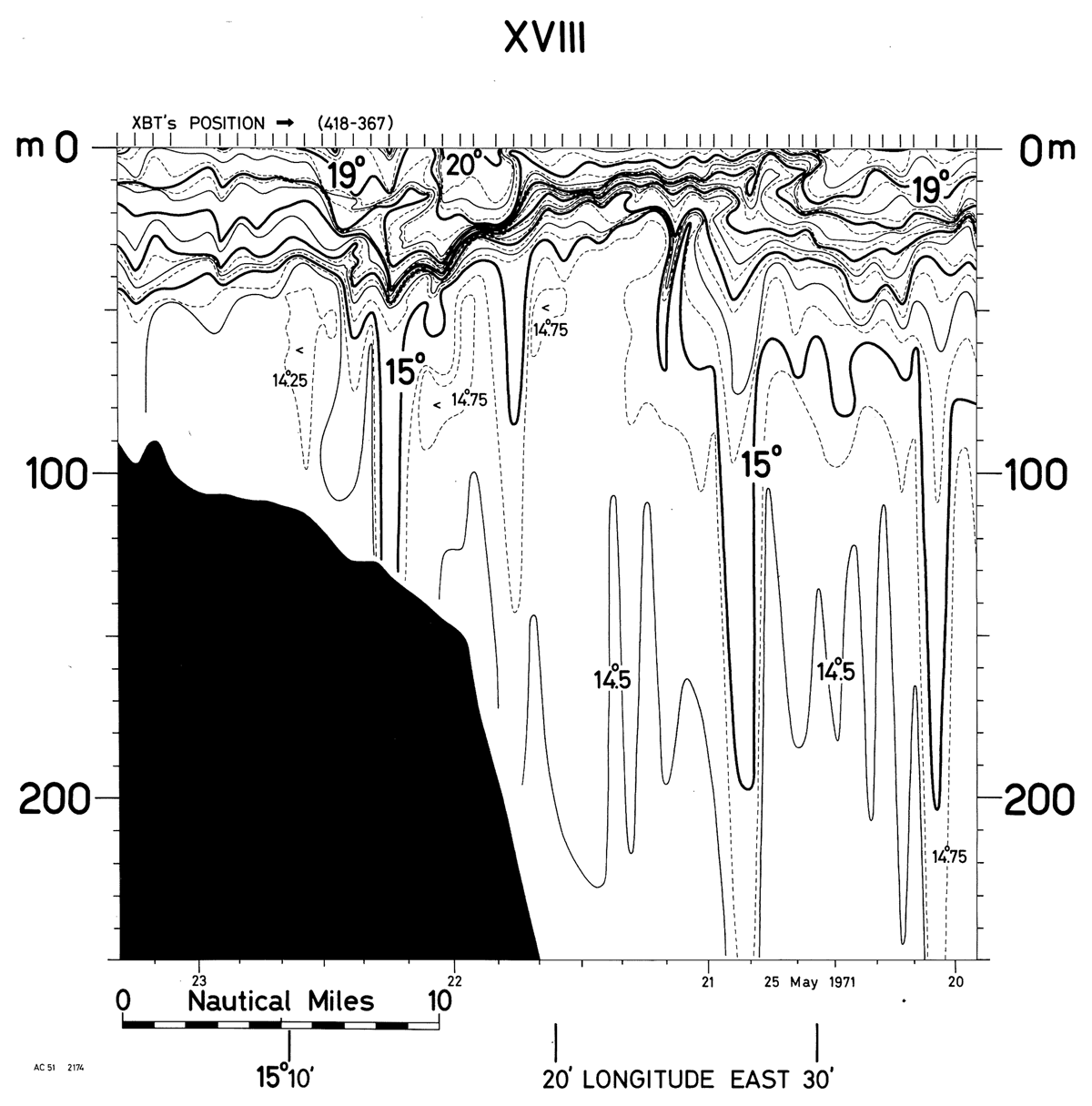
Figure 7
Expendable temperature probe (XBT) temperature section XVIII on 25 May 1971; for position, see Figure 5. [Source O. M. Johannessen].
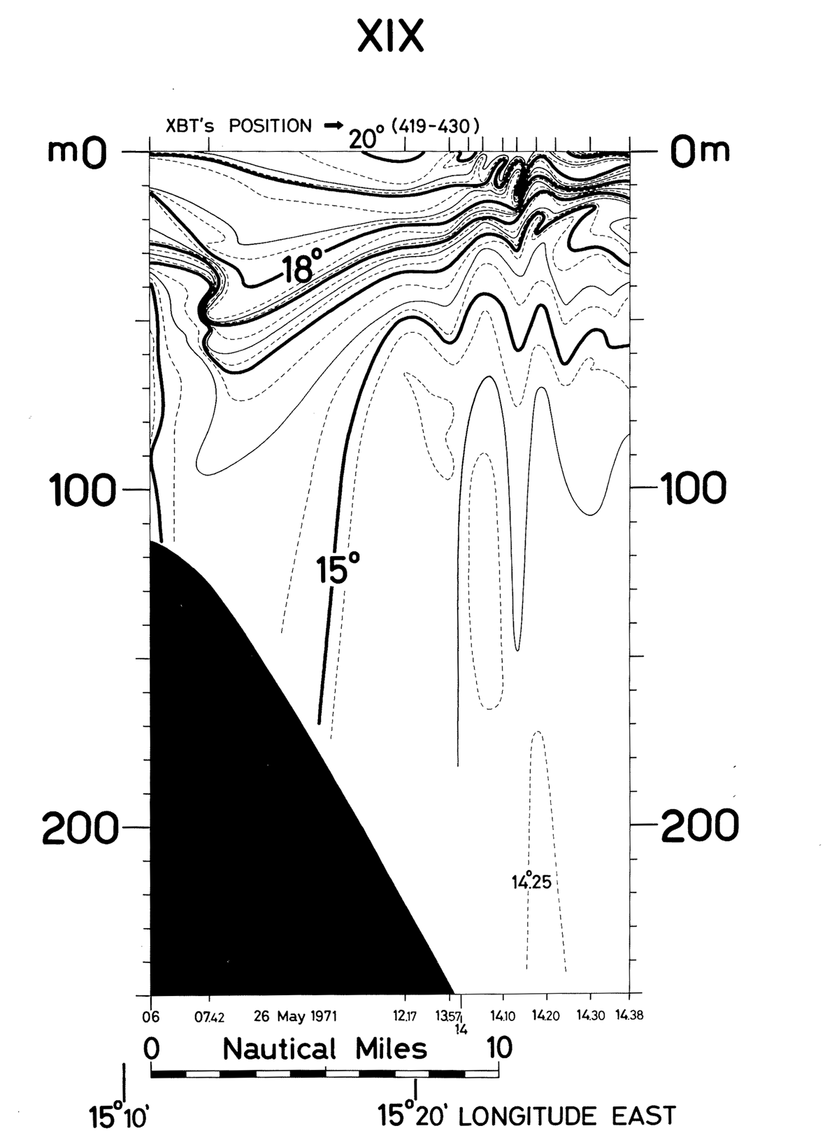
Figure 8
Expendable temperature probe (XBT) temperature section XIX on 26 May 1971; for position see Figure 5. [Source O. M. Johannessen].
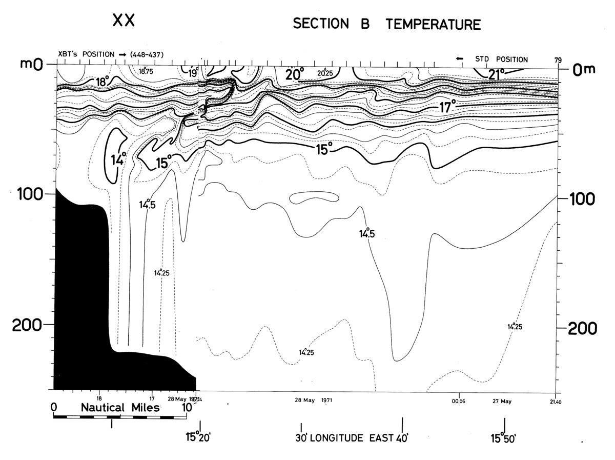
Figure 9
Merged temperature section STD Section B and XBT Section XX on 27–28 May 1971. [Source O. M. Johannessen].
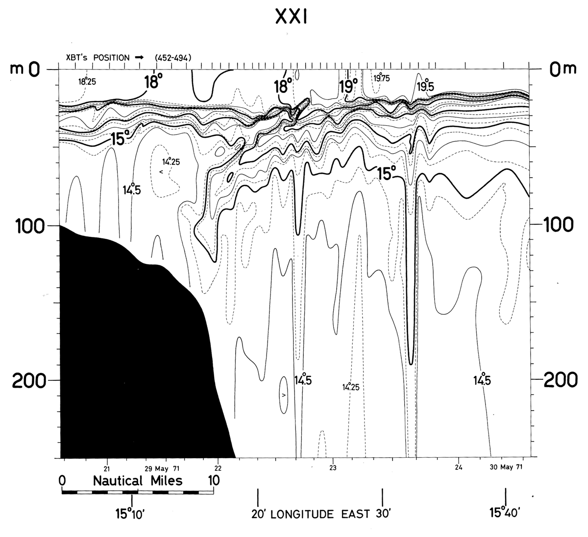
Figure 10
Expendable temperature probe (XBT) temperature section XXI on 29 and 30 May 1971; for position see Figure 5. [Source: Johannessen (1976), Figure 10].
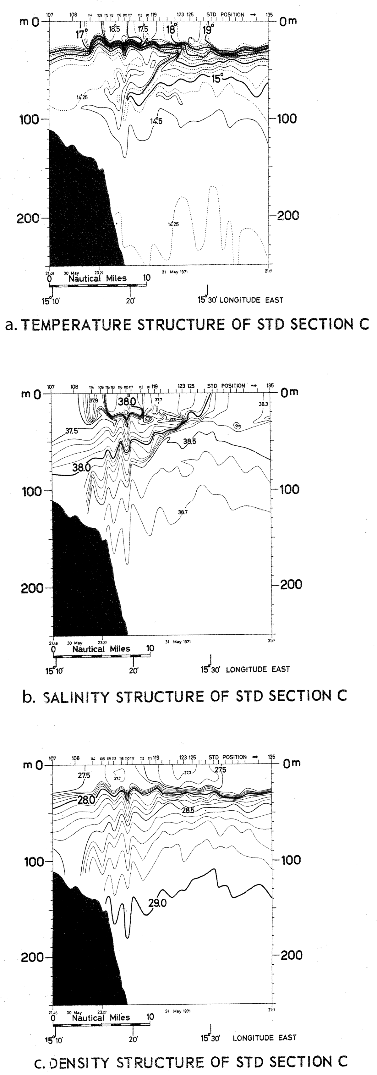
Figure 11
a, Temperature, b, salinity and c, density (STD) Section C on 30 and 31 May 1971; for position see Figure 5. [Modified after Johannessen (1976), Figures 10, 11, 12].
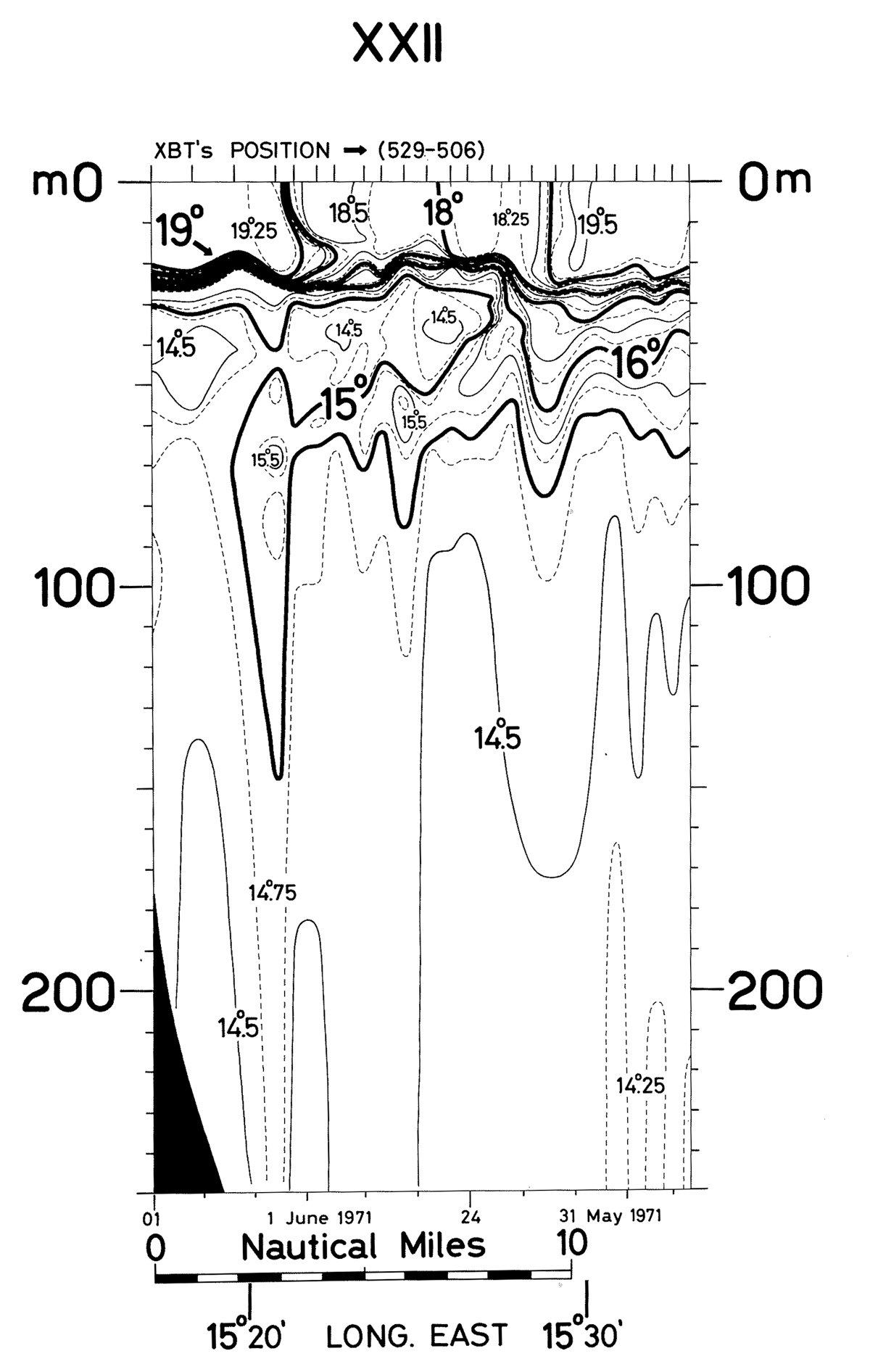
Figure 12
Expendable temperature probe (XBT) temperature section XXII 31 May and 1 June 1971; for position see Figure 5. [Source O. M. Johannessen].
4. Frontal Dynamics
The current meter array was anchored during the period 27–30 May for three days at 37°58’ N and 15°22’ E, marked in Figure 6a. The current meters were at five m in the upper layer, at 15 m at the top of the frontal interface, at 30 m just below the interface and at 60 m well below the frontal interface, see Section B/XX in Figure 9, which was observed after anchoring the current meter array on 27 May in the afternoon. The current meters recorded every five minutes, thereafter lowpass filtered with a 30-minute cutoff and decimated at 15 minutes, see Figure 13, which shows vector diagrams for each three hours. In Table 1, the mean daily current for the different depths is listed. The current is generally flowing southwards along the edge of the shelf with a speed in the surface layer at five m, varying daily between 41–53 cm/s, at 15 m between 38–46 cm/s, below the interface at 30 m between 31–33 cm/s and well below the interface at 60 m between 7–8 cm/s. These current observations are consistent with the model flow from Sicily towards the south along the shelf-slope off Malta (Pinardi et al., 2015) and the remote-sensing observations by Suarez et al. (2019). From day two to three, Table 1, the current increase in the surface layer with about 10 cm/s due to the strong wind from northwest but no significant change below the interface, thus resulting in a slightly stronger vertical shear and causing stronger internal variability below the pycnocline, breaking up the previously sharp frontal boundary (Figure 11).
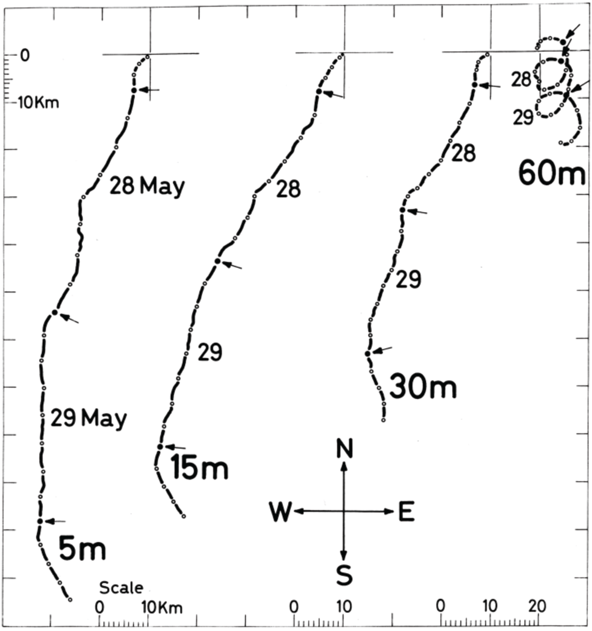
Figure 13
Vector diagram for current observations at 5–15–30–60 meters during 27–30 May 1971. Open dots indicate 3-hour interval, position marked on Figure 6. [Source: Johannessen (1976), Figure 9].
The current at 5 m and 15 m on 28 May (Figure 13), showed a weak semidiurnal tidal period (M2 = 12.5 hours), consistent with the M2 analysis by Agresti (2018) while at 60 m the flow is rotational in a clockwise direction with a period close to the inertial period of about 20 hours with a radius of about 4 km. The orbital current speed at 60 m is on the average 30 cm/s after removing the average flow. The formula for the inertial radius for inertial motion is R = U/f (U is the flow and f is the Coriolis parameter) when using U equal 30 cm/s which is the average flow for each 3 hours interval at 60 m, give R = 3.5 km, close to the observed value of 4 km in Figure 13. It should be mentioned that the spectra for the 15°C isotherm in the depth range 60–90 m for the internal wave observations clearly showed a peak at the inertial period with a minor peak of the semidiurnal tide, Chunchuzov et al. (2023).
The Rossby number R = V/f.L = 0.25 where V = 0.45 m/s which is the average speed in the upper layer during day 1 (Table 1) and L is 10 km, the amplitude of the width of the meandering front (Figure 4) and f the Coriolis parameter, indicating that the front was in geostrophic balance with a slope of 3.4 × 10⁻³ (Figure 6), at least before the strong wind started to change the mixed layer depth and the structure below, STD Section C (Figure 11). However, the slopes for the different section varied between 1.1–3.4 × 10⁻³ with an average value of 2.6 × 10⁻³. The surface of the frontal boundary varied between 15°26’–15° 30’ E longitude, which is 6 km, within the frontal width of 20 km shown in the ART SST mapping on May 19 (Figure 4). This suggested that the flow across this 36° N section varied in time due to the meandering of the propagating front, as also shown by the current observations (Figure 13, Table 1) and the upwelling and downwelling along the frontal interface.
As mentioned above, some local instabilities in the density structure were observed along the frontal interface (Figure 6c). However, the current observations and density profiles do not have high enough resolution to accurately calculate the Richardson number. Furthermore, the density profiles and the vertical shear were not observed at the same time. Therefore, we cannot rule out that shear instabilities can occur, probably caused by breaking of internal waves as observed off Malta by Woods (1968). D’Asaro et al. (2011, their Figure 4) also suggested that the wind forcing along a front including the Ekman transport across the frontal region caused instabilities and increased turbulence along the vertical frontal interface which could be a reason for the breaking up the frontal interface in Section C (Figure 11) during the strong wind event.
5. Discussion
In summary, this paper has described the legacy observations of the MAYFROST Experiment in 1971, the interpretation of the front’s location, its meandering structure, and some of its dynamics under calm and windy conditions including eddies that were spun off from the meandering frontal boundary.
In order to compare the Maltese Ocean Front with other fronts, two very detailed studies of ocean fronts in the eastern and western Mediterranean are considered here, in addition to the Nardelli et al. (2001) study mentioned in the Introduction. In 1970 from 5 to 11 December, a detailed investigation of an ocean front in the deep water of the Ionian Sea, located in a north-south direction at 17° E longitude was done. The study was carried out by using a 250 m long thermistor chain, Lafond and Moore (1962), towed by the R/V USS S.P. Lee of the Naval Undersea Research and Development Center, San Diego, California, and the use of an STD, under moderate wind condition (Johannessen et al., 1977). The thermistor chain had 45 thermistors, equally spaced with a system accuracy of 0.1°C, sampling every 10 s, low-pass-filtered giving values every 370 m in the horizontal. Some spectacular narrow mid-oceanic upwelling cases from the thermocline located at 60 m up to the surface were observed by the thermistor chain, which was towed for six knots, nearly synoptic across the front. The front was located over deep water and was not correlated with the topography, as the Maltese front was. In general, in an ocean front two water masses are converging but, in this case, a third subsurface water mass from the eastern Mediterranean was involved. This ‘Ionian Winter Ocean Front’, observed for the first time in this investigation, was dominated by pronounced upwelling of about 60 m with less downwelling of about 30 m. Geostrophic calculation of the current indicated that the horizontal shear was 5 times less than the Coriolis parameter. It was speculated that this relative high value of the horizontal shear, actually the vorticity, since cross-frontal movement was small, indicated that this was a region favorable for upwelling (Eliassen, 1966). These observations show that strong deep water mid-oceanic upwelling also can occur during wintertime when the mixed layer is about 60 m compared with the spring mixed-layer depth of 10–25 m in the Maltese Ocean Front.
Probably the most advanced ocean frontal experiment in the Mediterranean Sea up to date was done across the Almeria-Oran (AO) ocean front in the Alboran Sea in western Mediterranean in the CALYPSO project in 2018 (Zarokanellos et al., 2022). Here, gliders moving in parallel lines across the AO front resulted in 33 cross sections of ocean and biogeochemical structure; see their Table 1 for the type of gliders and the instruments on them. Furthermore, remote sensing of Absolute Dynamic Topography, SST and ocean color were observed in the experiment in order to provide a synoptic view of mesoscale structures such as meanders, eddies, and filaments in the frontal region, also including numerical simulation of the front. The experiment took place over a 2.5-month period starting in mid-May 2018. This integrated data set ‘indicated that vertical velocities in the AO can be developed by frontogensis, submesoscale activity, or by intrusion of cold filament in the study area’. Furthermore, the glider observations indicated ‘strong vertical motion on one or both sides of the AO front, and therefore high vertical fluxes can occur, which will enhance the phytoplankton biomass’, which was a focus of their study. Compared to the MAYFROST Experiment, the CALYPSO Experiment was a more advanced integrated frontal experiment, utilizing state of art modern technology including numerical simulations.
As mentioned before, ocean fronts are present in all world ocean and coastal areas, Mauzole (2022). The MAYFROST Experiment was a high-resolution case study both under very calm and windy conditions showing how a front respond to a sudden wind increase, perhaps one of rare events observed, modeled by Adamec and Garwood (1985) and in general by Mahadevan et al. (2010). The MAYFROST Experiment falls in the category of other high-resolution observations of ocean fronts, two already mention above in addition to the Nardelli et al. (2001) in the Mediterranean. Similar frontal experiments, to mention a few, have been carried out by LaFond and LaFond (1971) across the California ocean front, by D’Asaro et al. (2011) and by Zhu et al. (2024) in the Kuroshio Current region, by D’Asaro et al. (2018) in the northern Gulf of Mexico and the topographically controlled Oceanic Polar Front in the Barents Sea (Johannessen and Foster, 1978). Furthermore, in the ‘Review of oceanic front’ by Johannessen (1975), ocean fronts from many World Ocean, 57 examples, have been included from the first mesoscale investigations by Uda (1938) in the seas around Japan to the Maltese Ocean front by Briscoe et al. (1974).
What is novel about the MAYFROST Experiment is that the observations were obtained during a period of very calm wind period, where upwelling and downwelling along the sharp frontal interface took place. Furthermore, the response of the front to a sudden strong wind event along the front, with the denser water to the left, causing the mixed layer to increase its depth from 10 to 20–25 m, increasing the downwelling and ceasing the upwelling, breaking up the previous sharp interface and generate more internal variability below the thermo/pycnocline.
However, so far only one 2D temporal modelling of the Maltese Front has been done by Adamec and Garwood (1985) inspired by the detailed observations by Johannessen (1976). They focused on the study of the response of the frontal structure to the sudden strong wind event, initializing the model using the density structure from STD Section A (Figure 6c). However, they were not studying the upwelling and downwelling observed in this section under calm wind conditions, only the response of the front to the observed strong wind along the front. The model predicted the spreading of the isopycnals in the frontal boundary below the surface mixed layer as observed in STD Section C (Figure 11); however, the model overestimated the deepening of the surface mixed layer, which they predicted to increase with more than 20 m, while the observations only show about 10–15 m. They also predicted that inertial oscillations were generated when the wind stress was along the front. However, the observations of the inertial waves in this frontal region analyzed by Chunchuzov (2023) showed that the inertial waves were already present before the wind increased and that they were generated by both the front and irregularities in the bottom topography (Chunchuzov et al., 2023) and not by the wind as modeled by Adamec and Garwood (1985).
The MAYFROST observations of a meandering frontal wave with wavelengths between 15–30 km and a width of 20 km, propagating southward 2.1 km/day, with upwelling at the crests (Figure 4) and upwelling and downwelling under calm conditions, STD Section A (Figure 6) is consistent with the numerical modeling by Wang and Ikeda (1997) in their 3D model, with a resolution of 5 km in a rectangular long channel 125 km wide including a sloping bottom from west to east. They showed that up-welling occurred at the crests of the frontal wave, downwelling at the troughs and equal upwelling and downwelling at the nodes. The typical vertical speed was about 10 m/day, similar to the observations by Nardelli et al. (2001) in the northern part of the Maltese Front.
More recently, Mahadevan (2006) used higher resolution hydrostatic and nonhydrostatic numerical models than Wang and Ikeda (1997) to study ocean fronts, both for calm and windy conditions. The horizontal and vertical resolution were 0.5–1 km and 10–75 m, respectively, in a channel 48 × 96 km with a flat bottom, initialized by an idealized front with corresponding balanced velocities to study upwelling and downwelling in a meandering ocean front. Under no wind forcing, the simulated mesoscale upwelling and downwelling showed that the downwelling was 1.5 times more intense than the upwelling. When the models were forced by a constant wind stress along the front, intense sub-mesoscale vertical velocities developed in the upper 50 m, weaker below. Again, the downwelling was 1.5 times more intense than the upwelling, in both cases confined to narrow regions of about 2 km. Some of their modelling results are in general also seen in the observations of the Maltese front, e.g., that the downwelling is stronger under wind forcing (Figure 12). However, this is not the case for the no wind forcing, where the observations show that the upwelling was stronger that the downwelling at least at the crest of the frontal wave (Figure 6a). Furthermore the modelling results under no wind forcing observed a broad upwelling on the light side of the mesoscale meander similar to the ART SST map (Figure 4), see the review by Mahadevan (2016, their Figure 2b) which shows a schematic of a meandering front where up and downwelling are indicated. In the temperature Section 4 (Figure 9), the strong wind down-front had started to smear out the frontal boundary in the mixed layer due to the cross-frontal Ekman flux from the dense side of the front to the lighter side. Mahadevan et al. (2010) in a numerical model investigated the down-forcing of the wind along a front causing cross frontal Ekman flux from the dense to the light side, as indicated in Figure 9. They suggested that this mixing counters the re-stratification of the eddies which are generated along the frontal boundaries. This is observed in STD Section C (Figure 11), where an eddy is indicated on the light side of the front, without changing the depth of the surface mixed layer significantly. Recently, McWilliams (2019, see Figure 7, upper) has also dealt with upwelling along a straight frontal boundary ‘indicating a closed circulation loop with the upwelling on the light side and surface flow toward the dense side’. However, Figure 4 from the MAYFROST Experiment, shows that the upwelling does not occur all along the meandering front. For example, in the Maltese front, the upwelling is only indicated (Figure 4) to occur at the crests of the frontal wave. Further 3D realistic modeling of the Maltese Ocean Front may be interesting, using this legacy data set both for initializing and validation.
6. Summary and Conclusion
The meandering Maltese Ocean Front is located at the shelf-slope east of Malta with dominant horizontal wavelengths between 15 and 30 km with a wave width of 20 km, propagating southward about 2.1 km/day or 2.4 cm/s. The synoptic high-resolution surface temperature map indicates that upwelling was present at the crests of the frontal wave, including an eddy which was spun off the meandering front with a scale of about 20 km. The front was caused by the Atlantic inflow south of Sicily converging with the Ionian Sea water well correlated with the shelf-slope off Malta.
The frontal interface during calm wind condition was very strong, reaching from the surface to the bottom of the shelf with an east–west slope of 3.4 × 10⁻³. The Rossby number was 0.25 indicated that the front was in geostrophic balance, at least under calm wind condition. Stronger upwelling than downwelling was observed along the interface under calm wind conditions suggesting that this was near the crest of the frontal meander.
The frontal structure was significantly changed after a strong wind condition appeared. The surface mixed layer deepened by 10–15 m, also smearing out the outcrop of the front in the surface layer including strong internal wave activities below the mixed layer breaking up the interface, ceasing the up-welling but with enhanced downwelling indicating that this occurred at the trough of the subsurface frontal wave.
The current observations from the anchored buoy showed a flow a southward direction along the shelf-slope in the surface layer between 43–53 cm/s and below of 7–8 cm/s. During the strong wind period from northwest, along the front, the current speed increased by 10 cm/s in the surface layer but not in the deeper layer, causing an increase in the vertical shear. However the observations were to coarse to calculate the Richardson number. In the surface layer, a weak semidiurnal period was present, while in the lower layer the inertial period dominates, with clockwise orbital current speed of 30 cm/s with a radius of 4 km.
The observations from the Malta front are compared with some models, in particular Adamec and Garwood (1985), which is the only one dealing directly with this front. However, this model was 2D and only dealt with the response of the front to a sudden strong wind event, with some success, but not to the dominant upwelling and downwelling observed under very calm wind condition. Therefore, it is suggested that 3D modelling of this front should be done using these legacy detailed observations of the Malta Ocean Front both to initialize and verify model results.
The integrated case study of The Maltese Ocean Front reported in this paper, falls in the category of other high-resolution frontal investigations both in the Mediterranean and in other coastal and World Oceans. One unique result from the MAYFROST Experiment was perhaps that this front was, both observed under very calm wind conditions and, including the front’s response to a sudden strong wind event along the front, not often observed in other frontal regions.
Acknowledgements
Martin Miles is acknowledged for editing the paper and Tor I. Olaussen for preparing the figures. The reviewer is also acknowledged for useful comments improving the paper.
Competing Interests
The author has no competing interests to declare.