Improving Ocean Reanalysis with the Offline Ensemble Kalman Smoother

2.1 Ensemble Kalman smoother

The EnKF (Evensen, 2003) is a recursive ensemble-based data assimilation method. The ensemble of realizations of the model allows for a flow-dependent forecast error covariance estimate. A deterministic EnKF (DEnKF) variant has been developed by Sakov and Oke (2008). It uses a linear approximation of the theoretical error covariances to update the ensemble perturbations. This approximation yields a deterministic form of the conventional EnKF. In addition, compared to the traditional EnKF, the DEnKF inherently inflates the analysis error covariances by construction (Sakov and Oke, 2008).

Let the ensemble of model states at analysis time step ${\mathbf{\text{X}}}_{\text{f}}=[{\mathbf{\text{x}}}_{\text{f}}^1,{\mathbf{\text{x}}}_{\text{f}}^2,\text{…},{\mathbf{\text{x}}}_{\text{f}}^m]\in {\mathbb{R}}^{n\times m}$, the ensemble mean be ${\overline{\mathbf{\text{x}}}}_{\text{f}}\in {\mathbb{R}}^n$ and the ensemble anomalies or perturbations ${\mathbf{\text{A}}}_{\text{f}}={\mathbf{\text{X}}}_{\text{f}}–{\overline{\mathbf{\text{x}}}}_{\text{f}}{𝟏}_m^{\text{T}}\in {\mathbb{R}}^{n\times m}$, where the subscript ‘f’ denotes forecast, n is the size of model states, m is the ensemble size, and ${𝟏}_m={[1,1,\text{…},1]}^{\text{T}}\in {\mathbb{R}}^m$. The DEnKF update can be written as follows:

where the subscript ‘a’ denotes analysis, y is the observation vector, H is the observation operator that maps model states to the observation space, and H is the tangent linear operator of H. The Kalman gain K is defined by

where P_f is the forecast error covariance matrix estimated by the ensemble perturbations:

and R is the observation error covariance matrix.

We can rewrite Eqs. 1–3 into a form of the Ensemble Transform Kalman Filter as follows:

where T is the transform matrix (also known as X₅ in Evensen (2003)).

The (online/standard) EnKS is an EnKF extension (Evensen and van Leeuwen, 2000). It extends the analysis by adding the model state vector at the previous steps into X_f. In such a way, it updates the instantaneous model state that served as the initial conditions for the subsequent model integration and the model outputs in previous time steps.

The EnKS developed in this study is similar to the online/standard EnKS (Evensen and van Leeuwen, 2000) in that it incorporates future observations not used in the analysis, but does not require a model integration (black arrows in Figure 1). It is therefore numerically cheap. In this way, we can consider the EnKS method developed in this study as an offline approach (Raanes, 2016) or a post-processing approach to the pre-existing reanalysis (green dots in Figure 1).

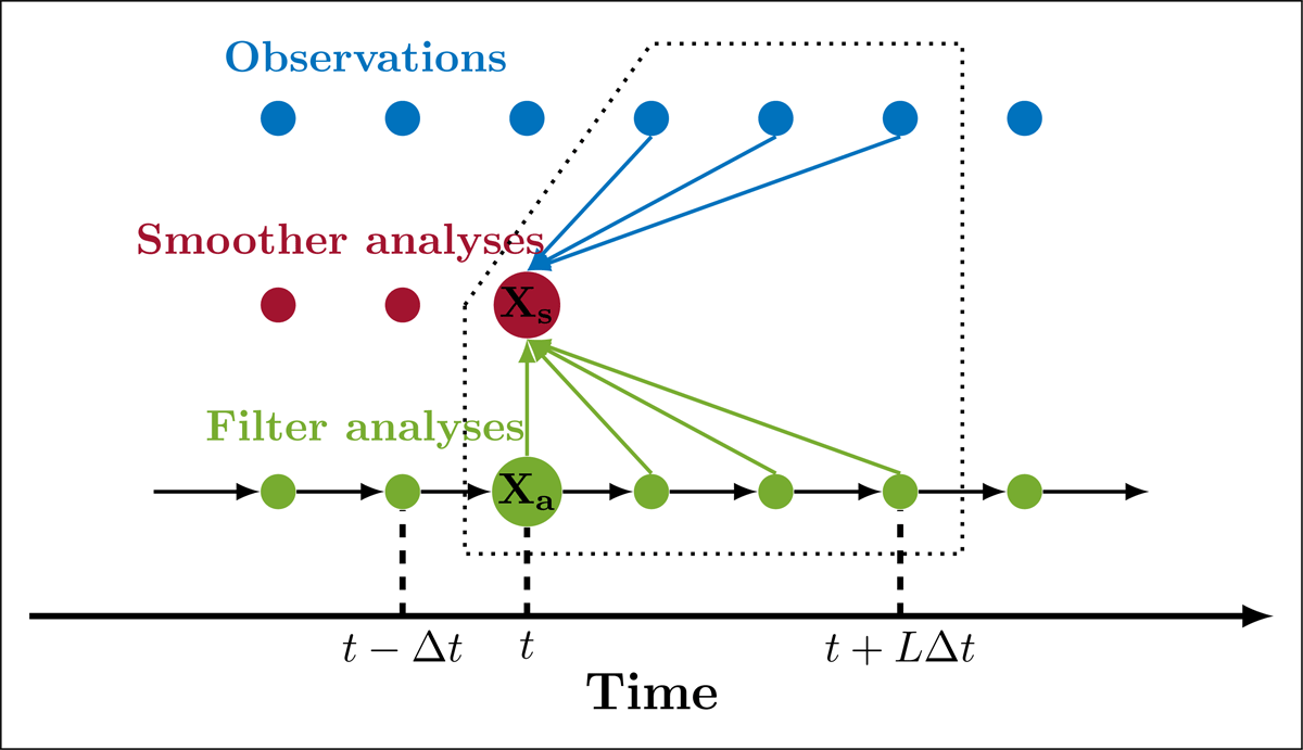
Figure 1

We propose to carry out the EnKS forward in time (i.e., sequentially from the first analysis to the last analysis) and consider a fixed lag of L time steps, meaning that the offline EnKS assimilates ‘future’ observations at L time steps ahead of time t. Please refer to the dotted shape in Figure 1.

We define the concatenated observations as

where y_k are observations at k time steps ahead of the existing analysis X_a at time t (Eq. 3) and $1\le k\le L$. Note that y₀ (i.e., y in Eq. 1) has been assimilated during the production of the filter analysis X_a and is not included in y_s for the smoother analysis. The concentrated observation error covariance matrix becomes a block diagonal matrix as follows:

in which observations from different times are assumed to be independent. The ensemble mean of the filter analyses within L time steps ahead of the model state X_a mapped to the observation space is written as

The tangent linear operator of the operator H_s is

The concatenated ensemble anomaly is defined as

The Kalman gain of the offline EnKS is written as

The offline EnKS can be written as follows:

For simplification, we can rewrite Eq. 16 as follows:

where T_s is the transform matrix (Evensen, 2003).

Note that the online/standard EnKS (Evensen and van Leeuwen, 2000) computes the transform matrix T (Eq. 7) based on the instantaneous model state X_f. We here compute the transform matrix T_s based on time-averaged model outputs of the reanalysis as it is costly to store for all instantaneous model states. In such a way, using the online/standard EnKS and our offline EnKS would lead to different solutions.

2.2 Test datasets

We apply the offline EnKS to two pre-existing NorCPM reanalysis datasets in an identical twin experiments and the real framework. NorCPM combines the Norwegian Earth System Model (NorESM, Bentsen et al., 2013) with the EnKF (Evensen, 2003) and has been developed to provide long-term coupled reanalysis (Counillon et al., 2016a; Bethke et al., 2021; Wang et al., 2022) and seasonal-to-decadal climate predictions (Counillon et al., 2014; Wang et al., 2019; Bethke et al., 2021). NorESM is a state-of-the-art global fully–coupled Earth system model for climate simulations and participates in the Coupled Model Intercomparison Project (Taylor et al., 2012; Eyring et al., 2015). It is based on the Community Earth System Model version 1.0.3 (Vertenstein et al., 2012), a successor to the Community Climate System Model version 4 (Gent et al., 2011). Its ocean component is the Bergen Layered Ocean Model (BLOM, Bentsen et al., 2013). Its sea ice component is the Los Alamos sea ice model (Gent et al., 2011; Holland et al., 2012). Its atmosphere component is a version of the Community Atmosphere Model (Kirkevåg et al., 2013). Its land component is the Community Land Model (Oleson et al., 2010; Lawrence et al., 2011). The version 7 coupler (Craig et al., 2012) is used. CAM4 and CLM4 have a horizontal resolution of 1.9° at latitude and 2.5° at longitude. BLOM and CICE4 have a horizontal resolution of approximately 1°. NorCPM comprises 30 ensemble members (m = 30 in section 2.1).

In the identical twin experiments (Halem and Dlouhy, 1984), the ‘truth’ is known and generated from the same model. We take advantage of the existence of simulations of twin experiments in Wang et al. (2022):

• – The truth has been spawned from the NorESM historical simulation by perturbing the sea surface temperature (SST) of the initial conditions in January 1960 with spatially uncorrelated white noise with a standard deviation of 10^{–6 ∘}C and then integrating it up to 2010.

• – Synthetic SST observations have been generated from monthly outputs of the truth with white noise. The noise amplitude has been set equal to the time-varying standard deviation of HadISST2 (Rayner et al., 2003) computed from its ten realizations.

• – The synthetic reanalysis of the NorCPM over the period 1980–2010 (Wang et al., 2022, its STEPmax simulation of twin experiments) has been produced by monthly assimilation of synthetic SST observations. This reanalysis has been produced with a vertical localization function that updates vertical layers down to the last layer for which a significant correlation with SST is found.

Please refer to Wang et al. (2022) for more details. These data (including the synthetic reanalysis, the truth, and synthetic SST observations) can be downloaded at Wang (2023).

In the real-world framework, we employ the offline EnKS technique on a 60-year coupled reanalysis dataset generated by the NorCPM model (Counillon et al., 2016b) and documented in Counillon et al. (2016a). This dataset spans from 1950 to 2010 and assimilates monthly SST observations from the HadISST2 dataset (Rayner et al., 2003) through the EnKF (Counillon et al., 2016a). It uses an anomaly assimilation framework that assimilates observational anomalies for the climatology period from 1950 to 2009. The observation uncertainties are defined as the standard deviation of ten realizations of HadISST2. It is essential to highlight that the reanalysis employed here has been rigorously validated. As detailed in Counillon et al. (2016a), this reanalysis has demonstrated considerable reliability compared to independent measurements, including assessments of sea surface height (SSH), ocean heat content, and ocean salt content. Furthermore, this reanalysis is reliable in providing accurate estimations of critical oceanic indicators, such as the North Atlantic Subtropical Gyre index and vertical temperature variability. Additionally, it has shown promising results in simulating the Atlantic Meridional Overturning Circulation. Please refer to Counillon et al. (2016a) for more details.

Note that the data assimilated in the offline EnKS (section 2.1) are the same monthly SST data used in the pre-existing reanalyses in Wang et al. (2022) and Counillon et al. (2016a).

2.3 Practical implementation and experiment setups

The EnKS, like many other ensemble-based data assimilation methods, relies on background error covariances to incorporate observed information into the model state (section 2.1). To mitigate the impact of spurious covariances due to sampling errors and small ensemble size, one commonly uses localization (Hamill et al., 2001; Houtekamer and Mitchell, 2001).

Localization is crucial for achieving optimal results of the EnKS (e.g., Khare et al., 2008). The appropriate choice of localization parameters, such as the spatial extent of the localization function or ‘localization radius’, depends on the specific characteristics of the model and the observations. Overly aggressive localization, such as setting a very short localization radius, can lead to the underutilization of available observations. In such a case, the assimilation process becomes excessively conservative and fails to effectively integrate observed data into the model, resulting in less accurate state estimates. Conversely, an overly large localization radius allows spurious variability to introduce artificial signals into the assimilation process. This can lead to the incorporation of noise or irrelevant information, potentially deteriorating the quality of the state estimates.

We use a local analysis framework (Evensen, 2003; Hunt et al., 2007). The smoother analysis uses the neighboring local observations (in space and time). To effectively account for the influence of distant observations in space, we adjust the observation error variance by applying the reciprocal of the Gaspari and Cohn localization function (Gaspari and Cohn, 1999) as in NorCPM. As demonstrated by Sakov and Bertino (2010), this approach is equivalent to utilizing the localization function to filter for the background error covariances. The spatial localization radius is a bimodal Gaussian distribution that varies with latitude (Wang et al., 2017). It is smaller in high latitudes compared to mid-latitudes to account for the Coriolis force’s effects. The localization radius reaches a local maximum of approximately 2300 km at mid-latitudes and decreases to around 1500 km near the Equator to account for the anisotropy of the covariance there.

For the temporal localization, we employ the reciprocal of an exponential function γ^l for tapering observation error variances, such that γ accounts for the decay rate per month (representing the assimilation cycle), and l denotes the time lag in number of months within three months (i.e., L = 3 in section 2.1 and Figure 1). This temporal localization function has demonstrated its utility in prior studies, such as Dong et al. (2021), where it contributed to the enhancement of daily high-resolution ocean reanalysis, as well as in the Lorenz 1963 idealized system examined by Dong et al. (2023). In our twin experiments, we perform 6 experiments, with temporal parameters $\gamma =0.01,0.05,0.1,0.2,0.3,\text{or} 0.5$. To provide some insight on the delay timescale, we make use of the formulation $–\frac{1}{\text{ln}(\gamma )}$ from Dong et al. (2023). The chosen temporal parameters correspond to a delay timescale of 6.5, 10.0, 13.0, 18.6, 25.0, and 43.0 days.

As the process of producing a gridded product from sparse observations introduces correlation in the observation error, in the real framework, we multiply observation error variance by a factor of 1, 2, 4, 6, 8, 10, 16, or 25 to take into account observation correlation as suggested in Stewart et al. (2008). We conduct 8∗6 (i.e., 48) experiments in the real framework, considering both correlated observations and temporal parameters.

In all experiments, the offline EnKS updates monthly data for SSH, mixed layer depth (MLD), and temperature and salinity for all depth levels of the reanalysis.

2.4 Validation datasets

We use the truth to validate the smoother analyses in the twin experiments. In the real framework, we use the EN4.2.1 objective analysis dataset (Good et al., 2013) to validate anomalies of top 300 m temperature (T300) over the period from 1950 to 2010. For SSH, we estimate anomalies from 1993 to 2010 using the gridded dataset ARMOR-3D L4, which can be accessed at https://doi.org/10.48670/moi-00148. The MLD dataset is available from 1958 to 2010 and taken from the ORAS5 global ocean reanalysis at https://doi.org/10.24381/cds.67e8eeb7. All these datasets are independent of the SST dataset assimilated into the system (i.e., HadISST2).

2.5 Evaluation metric

We use the mean squared skill score (MSSS, Murphy, 1988) to evaluate the smoother analysis. We take the original (or filter) analysis as the reference to define the MSSS as follows:

where MSE_f (MSE_s) is the mean squared error of the filter (smoother) analysis against the truth or independent observations. A positive (negative) MSSS value indicates that the smoother analysis is more (less) accurate than the filter analysis. If MSE_s is equal to zero (i.e., the smoother analysis is perfect), the MSSS is equal to one. It is worth noting that the MSSS is equivalent to the squared error reduction ratio.

Before the MSSS computation, the reanalysis and the (independent) validation data are interpolated to a common regular $5^{\circ }\times 5^{\circ }$ grid. We evaluate the top 300 m temperature (T300), SSH, and MLD, which are highly relevant to climate studies. We also verified other quantities, such as the top 300 m salinity (S300) and temperature below 300 m, but improvements were either weak or none (please refer to Figure 1 in Supplementary Information).

To check the reliability of the reanalysis, we made use of the assimilation diagnostics proposed by Desroziers et al. (2005) and used in many applications (e.g., Bethke et al., 2018; Counillon et al., 2016a; Sakov et al., 2012; Slivinski et al., 2021). We define global statistics as follows:

where w_i is the area of grid cell i relative to the global ocean area, d_i is the difference between observation and reanalysis, ${\sigma }_i^r$ is the standard deviation of the ensemble of reanalysis representing reanalysis error, and ${\sigma }_i^o$ is observation error. d represents the root mean squared error (RMSE) computed over the difference between the observations and the reanalysis. $\overline{{\sigma }^r}$ and $\overline{{\sigma }^o}$ represent the globally-averaged reanalysis and observation errors, respectively. According to Desroziers et al. (2005), in the case where the observation and reanalysis errors are uncorrelated and unbiased, the RMSE d is expected to be equal to the combined error σ, meaning the reanalysis is reliable. Since the reliability budget relies on the observation errors or uncertainties often not provided in the datasets, we only check the reliability of the reanalysis for SST (i.e., the assimilated quantity).

3.1 Twin experiments

All temporal parameters yield positive MSSS values for monthly T300, SSH, and MLD (Figure 2), underscoring the promising potential of the offline EnKS method. However, the improvements vary with the temporal localization parameter γ. The optimal results are obtained with γ = 0.1 for all three quantities, corresponding to a delay time of 13 days. Higher or lower temporal localization degrades performance, revealing that the smoother timescale at the ocean surface is less than one month – in close agreement with the findings in Dong et al. (2021). Assimilating future SST data is slightly more efficient for T300 (13%) and MLD (12%) than SSH (10%, Figure 2). We show only the experiment results with γ = 0.1 in the rest of this section.

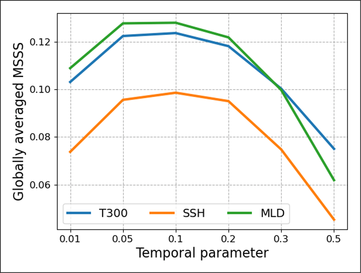
Figure 2

For monthly T300, we find larger errors near the Equator and western boundary currents (Figures 3a), where the improvements (or error reduction) from the offline EnKS with the optimal parameter are evident. We also find prominent improvements in the Southern Ocean along the Antarctic Circumpolar Current, the largest wind-driven current on Earth. In these regions, dynamics are chaotic, and errors evolve quickly. Future observations can help to constrain state errors effectively.

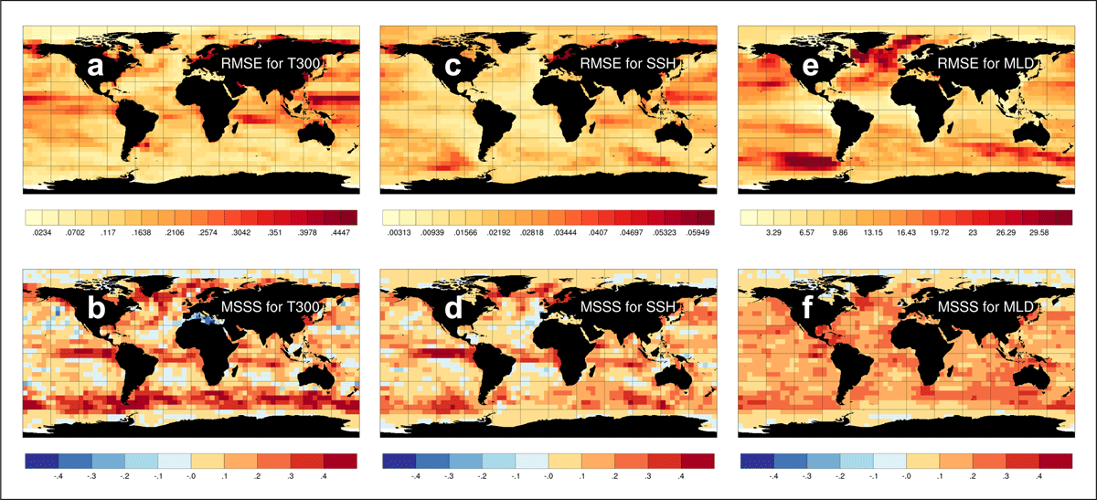
Figure 3

SSH variability encompasses a broad range of factors, making it a comprehensive metric for capturing changes in ocean conditions. It reflects both steric and dynamic alterations within the oceanic system. SSH variations are closely related to the thickness of the upper layer and thermocline-depth variations in the tropical regions (Wyrtki and Kendall, 1967). The patterns of RMSE in monthly SSH are similar to those of T300 (Figure 3c) due to the contribution of thermosteric changes, except for the Southern Ocean, where dynamic changes play a key role in SSH variability. SSH exhibits MSSS scores slightly lower than T300, but their spatial patterns exhibit remarkable consistency (Figures 3b,d).

Ocean stratification is mainly driven by temperature in most places, and salinity plays a role in the high latitudes. We find large RMSEs in MLD in the North Pacific, North Atlantic, and Southern Ocean (Figure 3e). These regions extend into higher latitudes with a greater contrast in temperature between the surface waters and the deeper ocean. This contrast promotes vertical mixing, especially in winter, and contributes to a deeper MLD. In addition, ocean currents and gyres, such as the Antarctic Circumpolar Current and the North Atlantic Subtropical Gyre, lead to changes in the ocean’s vertical structure, deepening the mixed layer. Figure 3f shows that the assimilation of future SST data with the offline EnKS significantly reduces the error in monthly MLD. The MSSS score is globally homogeneous, except for sea ice cover regions where SST data is not used.

The offline EnKS significantly improves the reliability of the reanalysis for monthly SST. Figure 4 shows that the filter analysis has a larger combined error σ^f than the RMSE d^f. The offline EnKS reduces both the combined error σ and the RMSE d, but the reduction of the combined error is more prominent. It makes the two quantities, the combined error and the RMSE, closer in the smoother analysis, meaning the reanalysis becomes more reliable (Desroziers et al., 2005).

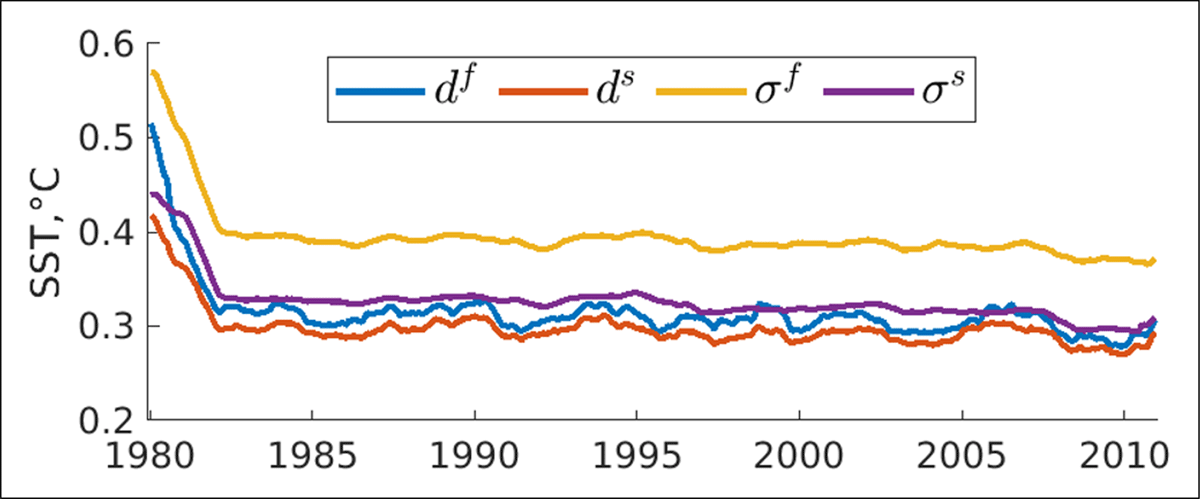
Figure 4

Essentially, the offline EnKS uses an ensemble of pre-existing filter analyses to capture and represent the temporal relationship (i.e., covariance) between model states at different time steps and to correct and improve the filter analyses with future observational data. This approach enhances the accuracy of the reanalysis, particularly in regions where ocean currents are active and the error is large. Also, the reliability of the reanalysis is improved.

3.2 Real framework

It is important to note that, unlike in the above twin experiments, where the model was perfect, the Earth system model often has a large model bias. We calculate the scores in the anomaly field within the real framework, meaning the validation process does not consider model biases.

We tested different temporal localization parameters for the twin experiments (section 2.3). Several combinations of temporal localization parameters and observation error inflation factors lead to a similar performance (not shown in this paper). The larger the temporal localization parameter γ, the more we need to inflate the observation error. In the following, we use the temporal localization parameter γ = 0.1 to be consistent with section 3.1.

When validating on the monthly timescale in the real-world framework, we find the positive MSSS values for monthly T300, SSH, and MLD anomalies in most grids (please refer to Supplementary Information) but notably lower than those in twin experiments. Potential factors causing this inconsistency will be discussed in section 4. In the following discussion, we show the results on the yearly timescale, meaning the validation for yearly T300, SSH, and MLD anomalies.

Overall, the offline EnKS yields positive globally averaged MSSS values in all realistic experiments for the three quantities (Figure 5). The improvement (or error reduction) is larger for MLD and lower for SSH, which is consistent with the results in the twin experiments (Figure 2). However, it is moderate for T300, which is inconsistent with the results of the twin experiments (Figure 2). It may be because sparse hydrographic profile measurements before the Argo float period (2000s) led to high uncertainties in the EN4 Objective Analysis (i.e., the reference dataset).

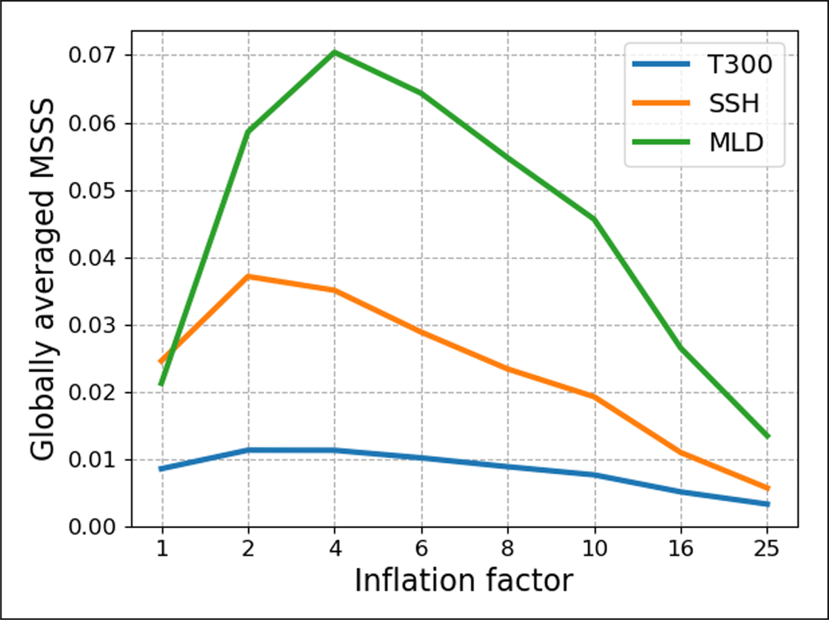
Figure 5

Note that the inflation of observation error variance (Stewart et al., 2008) was designed to neutralize the fact that the errors of actual observations are correlated. According to overall MSSS values in Figure 5, we have to inflate observation error variance by four times to reach the optimal performance of the offline EnKS.

For yearly T300 anomalies, the large RMSE is found in the regions aligning with the ocean currents, e.g., the Gulf Stream and Agulhas current (Figure 6a). The offline EnKS leads to positive MSSS values in the regions with larger RMSE (Cosme et al., 2010), but negative MSSS values in some other regions (Figure 6b).

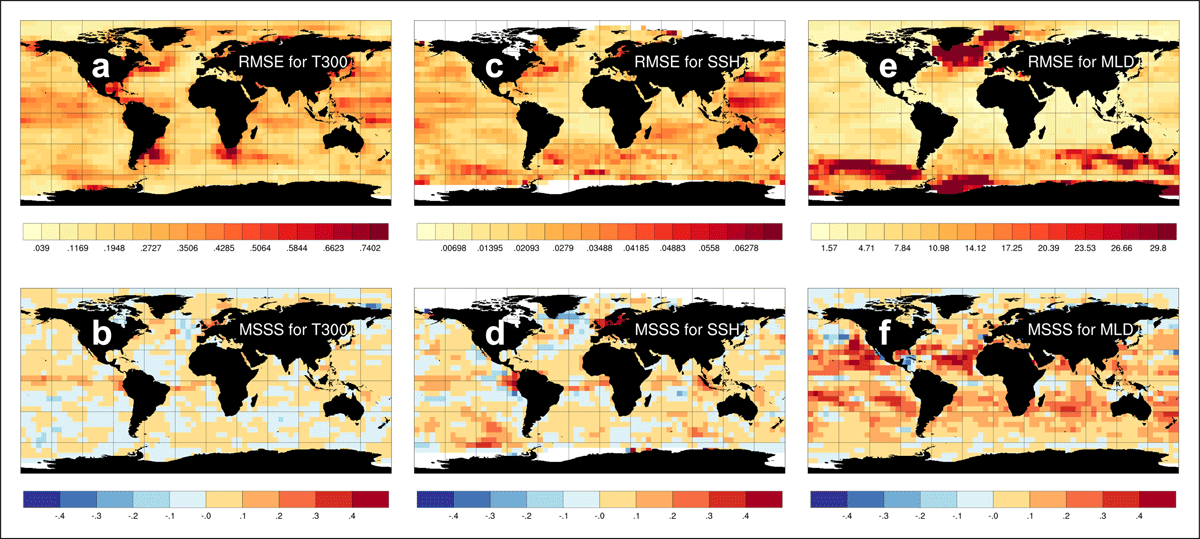
Figure 6

For yearly SSH anomalies, the spatial pattern of RMSE (Figure 6c) is similar to T300 anomalies (Figure 6a), except for the Southern Ocean, where ocean dynamic is a key factor for SSH variability and the quality of EN4 Objective Analysis is questionable. The magnitude of the MSSS values is larger than T300 anomalies (Figure 6). Many other factors influencing SSH variability, in addition to T300 anomalies, are improved by the offline EnKS. Furthermore, SSH observations have only been available since 1993, and the MSSS of T300 anomalies was computed from 1950 to 2010. Their validation periods are different.

For yearly MLD anomalies (Figures 6e-f), significant errors are found in the North Atlantic Subpolar Gyre region, Norwegian Sea, Southern Ocean, and the Weddell Sea where deep convection occurs (Courtois et al., 2017). The positive MSSS scores are found in most regions, particularly subtropical areas. Overall, the improvement in MLD is more prominent than in T300 and SSH, consistent with Figure 5.

The offline EnKS improves the reliability of the reanalysis for monthly SST anomalies. Figure 7 shows the time series of the RMSE d and combined error σ for monthly SST anomalies in the filter and smoother analyses. The discontinuity in the combined error σ in the 1980s is due to the availability of satellite data dramatically increasing the quality of observations. While the offline EnKS reduces the RMSE d, the combined error σ decreases. Regarding reliability, in the satellite era, d and σ match better in the smoother analysis than in the filter analysis.

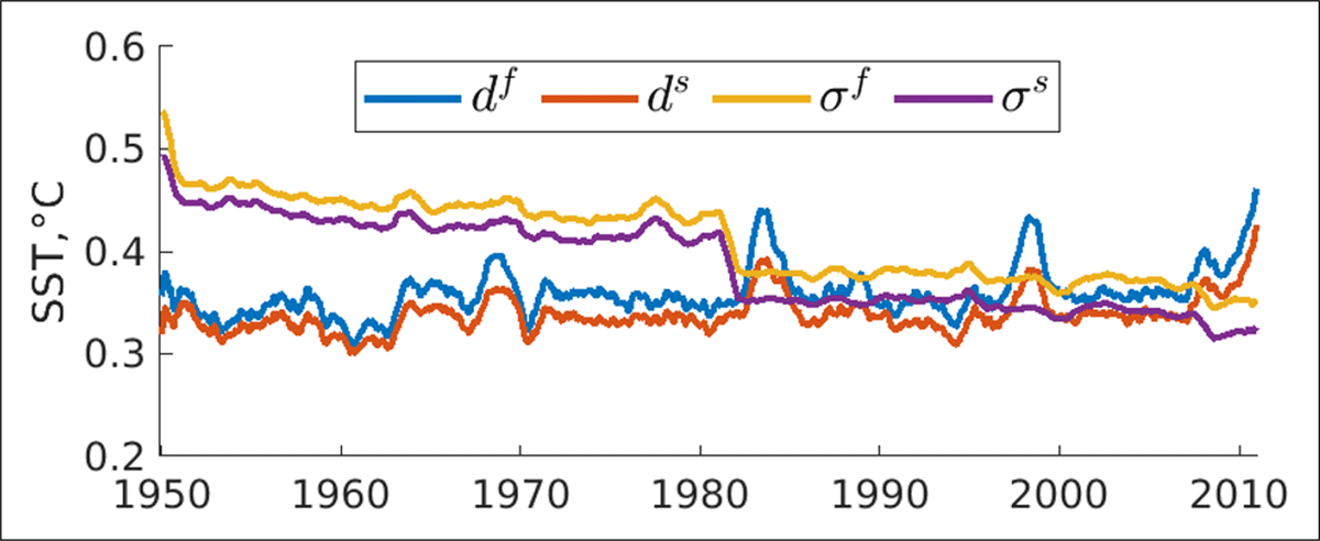
Figure 7